Cloud Computing -- Google Docs Way: yogi_Conditionally Format B1:D1 When Date In Column A Is TODAY And Columns B:D Houses Off In Any Row

Sunday, August 5, 2018

yogi_Conditionally Format B1:D1 When Date In Column A Is TODAY And Columns B:D Houses Off In Any Row

Google Spreadsheet Post #2482

Yogi Anand, D.Eng, P.E. ANAND Enterprises LLC -- Rochester Hills MI Aug-05-2018

question by: Cary K
https://productforums.google.com/forum/?utm_medium=email&utm_source=ba_notification#!topic/docs/guf_6HBhZT4;context-place=forum/docs
Conditional formatting - Changing header cell color if two cells in row match criteria

Hi All!

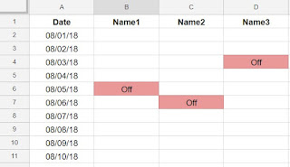
I'm hoping someone can help me with a problem I'm having because it's definitely stumped me. I consider myself to be pretty proficient with conditional formatting but am struggling trying to figure out how to change a header color based on the values of two cells in a row. I have Names as headers (Row 1) and Dates in column 1. The dates would actually be a list of all the dates in a calendar year. In this example, I've just included a few from August.

What I'd like to do is when the date in column A equals today's date AND the value in the cell in column B for today's date is equal to "OFF", I'd like to have the Name1 header change to a specified color. Same for Name2, Name3, etc if the value in their respective columns is "Off" and the date is today. So as an example if today's date was 08/05/18 and the value in column B for that date was "Off" then the Name 1 header would change color. Kind of like a intersection of the date and name if it's OFF.

I tried using =AND($A2=TODAY(),$B2="Off") in the "Custom Formula" portion of conditional formatting with the range being B1 but that didn't work. Same with the following ...

=AND(A:A=TODAY(),B:B="Off")

=AND($A1:A=TODAY(),B1:B="Off") as well as other formulas but none seem to work.