yogi_Set Up Array Formula With Open Ended Range For Finding The Current Trend In A Sheet

                                          Google Spreadsheet   Post  #1312
Yogi Anand, D.Eng, P.E.      ANAND Enterprises LLC -- Rochester Hills MI     www.energyefficientbuild.com.   Jul 30, 2013
user  theillway (http://productforums.google.com/forum/?zx=gx080770b9kk#!mydiscussions/docs/dpamcy2XFwU)
Finding the current trend in a sheet
I keep a spreadsheet of how much I have charged a client, and how much time I spent on work for that client.  I use this information to get the average of how much per hour I am charging.  I then use the trend function to figure out whether I'm improving or holding steady.  The problem is, everytime I enter in new information, I have to manually update which cells the trend should apply to (if I simply have the trend for the whole column, the formula breaks).  I want to be able to lock the sheet so that I can have other (less tech savvy) staff use the spreadsheet without fear.

I've tried messing around with lookup functions, but I haven't had any luck.  Right now, my trend formula is =TREND(G34:G57,A34:A57). I just need a way for the "57" to update to "58" if there is data in 58.

---

Here is a mock-up of the sheet I'm working on:

https://docs.google.com/spreadsheet/ccc?key=0AqvYpCphh7l9dDI0eXlQMmdJM1V4STV6TnV3RXBJMVE&usp=sharing

As you can see, for the last two entries, the trend column hasn't updated itself.

Otávio, I tried your formula, but it said a circular dependency was detected.

Yogi:

a) I thought it would be a simple matter to change "F34:F56" to something like "F34:(formula)".

b) I'm looking to have the trend be in column G.

c) Expected result is to have the trend automatically calculate in the same way that I have the hourly rate calculate itself.  So, a new client pays us, I put in the amount and the time worked, and the spreadsheet figures out the hourly rate and the trend.

Thanks in advance for the help.

-------------------------------------------------------------------------------------------------------------------------------------------------------

yogi_Pull Data From Select Columns of Sheet1 For Matching Location

                                          Google Spreadsheet   Post  #1311
Yogi Anand, D.Eng, P.E.      ANAND Enterprises LLC -- Rochester Hills MI     www.energyefficientbuild.com.   Jul 29, 2013
user  nerfsmurf (http://productforums.google.com/forum/?zx=6q0rj6nbkpey#!mydiscussions/docs/rgB2B0udwd8)
Displaying multiple values of cells within a column if a certain text value is in same row.
Good morning everyone! 

Made the title as specific as I could! Here is the complete version.

I have a Google form that give every row a category within a spreadsheet, lets use for example, "Store Name" in Column B. and B2:B900 can have either value "Store A", "Store B" or "Store C".

Also within the same Google form, there is a comment section. So in the spreadsheet, a row will include the name of the store and a few columns over, the comment.

I'm trying to list the data on a new sheet as follows: Column A will have all comments from store A, Column B will have all comments from store B and Column C will have all comments from store C.

I am currently using:

=iferror(INDEX('Form Responses'!$S$2:$S$902, MATCH(0, COUNTIF(C$23:$C24,'Form Responses'!$S$2:$S$902), "0")))

S is my comment column and C is my destination column where I need the data displayed.

I drag this formula down about 50 rows so I can see 50 comments, and it works except that it shows all comments. I have tried to fuse the FILTER function in there but with no luck.

Can anyone help?

-------------------------------------------------------------------------------------------------------------------------------------------------

yogi_MultiConditional Count -- Number Of Entries For A Specified Name In A Specified Range Of Dates

                                          Google Spreadsheet   Post  #1310
Yogi Anand, D.Eng, P.E.      ANAND Enterprises LLC -- Rochester Hills MI     www.energyefficientbuild.com.   Jul 27, 2013
user  Rajesh Iyery (https://productforums.google.com/forum/#!category-topic/docs/spreadsheets/lGLxjl5_lfk)
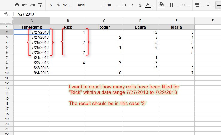
CountIFs query for Google Spreadsheet

Hi,

I have a spreadsheet and i want to count the filled cells of specific persons by a specific date range.  Please check the screenshot below and let me know your suggestion

---------------------------------------------------------------------------------------------------------

yogi_Split Row on New Line For All Entries In Column A Down From Row 2

                                          Google Spreadsheet   Post  #1309
Yogi Anand, D.Eng, P.E.      ANAND Enterprises LLC -- Rochester Hills MI     www.energyefficientbuild.com.   Jul 27, 2013
user  Justin Duffy (https://productforums.google.com/forum/#!category-topic/docs/spreadsheets/puzvclXEGlI)
Split rows based on new line
Hi all,

I have a spreadsheet that is importing a lot of data into rows.   I need to split these rows every time there is a new line character, creating an output like the one below:

Input	Output
This is the first item. This is the second one Sometimes the items end in a period. Sometimes they don't	This is the first item.
This is item 5 This is item 6 etc.	This is the second one
Item 7...	Sometimes the items end in a period.
	Sometimes they don't
	This is item 5
	This is item 6
	etc.
	Item 7...

Can you do this with the SPLIT function, or do you need to write a script?  Either way I am striking out, and would appreciate any help I can get.  A sample spreadsheet is here:

https://docs.google.com/spreadsheet/ccc?key=0AgLFdRWHtdTZdGZObHdkRldkZ3RTTEI4X0E5TnBVVEE&usp=sharing

Any and all help is appreciate!  Thanks in advance!

----------------------------------------------------------------------------------------------------------------------------

yogi_WorkAround For Querying Data When Source Data Has Field(s) With Mixed Data (Numeric and Text)

                                          Google Spreadsheet   Post  #1308
Yogi Anand, D.Eng, P.E.      ANAND Enterprises LLC -- Rochester Hills MI     www.energyefficientbuild.com.   Jul 26, 2013
user Jared Hamilton (http://productforums.google.com/forum/?zx=hmnbrbxx6547#!category-topic/docs/spreadsheets/m8CsEJyIHKE)
Spreadsheet Query problem

I was creating a spreadsheet to save our school dismissal person some time which is located here.  All data should be entered in "All Dismissal" then feeds out to appropriate tabs by Query.  My equation on the second sheet "3:15 Bus" is =QUERY('All Dismissal'!A2:I264,"Select B,C,D,E,F where I = '3:15 Bus' order by F")

My problem is that the query being made from the "3:15 Bus" sheet is only pulling the F column from the "All Dismissal" sheet when it is a number.  If anything other than a number is put in the F Column of "All Dismissal" then that column comes up blank in the "3:15 Bus" sheet.  I highlighted 2 examples in the spreadsheet.

---------------------------------------------------------------------------------------------------------------------------------------------

The problem is that column F in the source data (sheet named All Dismissal) has mixed data (Numeric and Text) ... QUERY function expects a field to have the same data type in its entirety ... so I used a WorkAround as presented in the following

yogi_Set Up A Calendar For List Of Days Of Specified Day of The Week In Months Of A Year

                                          Google Spreadsheet   Post  #1307
Yogi Anand, D.Eng, P.E.      ANAND Enterprises LLC -- Rochester Hills MI     www.energyefficientbuild.com.   Jul 25, 2013
user Paul Winn (http://productforums.google.com/forum/?zx=lhbkt93evv10#!category-topic/docs/spreadsheets/m0xWUgZ6sVM)
Specific dates for all Sundays in a month
I have a simple church schedule workbook with sheets for every month.  The 3 column headings are Date, Sound, Video.  Under the last 2 columns there will be just names of people assigned for either sound or video.  Since church is on every Sunday in a month, I would like to calculate the specific dates of the the 4 or 5 Sundays (and place them in 4 or 5 cells/rows beneath the "date" heading) for the corresponding month an year.  Maybe it is easier to just look at a calendar and copy the values but if there is a better way I'd love to know.
Thanks
----------------------------------------------------------------------------------------------------------------------------

yogi_Compute Row By Row Sum Of Two Columns Of Lap Times In Minutes Seconds And Milliseconds

                                          Google Spreadsheet   Post  #1306
Yogi Anand, D.Eng, P.E.      ANAND Enterprises LLC -- Rochester Hills MI     www.energyefficientbuild.com.   Jul 25, 2013
user Rick Robinson-Donnelan (http://productforums.google.com/forum/?zx=lhbkt93evv10#!category-topic/docs/spreadsheets/SN8LklEo7_Q)
adding two lap times together (MM:SS.000 milliseconds)
Hi guys

I've done a bit of searching but not been able to find the answer I was looking for.

Basically, I have two lap times (think racing) in the format of:

MM:SS:000 (tenths, hundreds, thousands)

so for example 1:37.456 

I then have another lap time, 1:37.978

I want to be able to add the two times together and come up with the total race time. Every time I do it, it comes up with a bad value and I can't see any option for it in the formatting. I know it must be easy to do but I don't know how.

1 rule however: The two lap times must be simple i.e. I need to be able to just type/copy and paste the numbers in without any formatting and then the Total field work out the rest for itself. I don't want to have to enter formulae into both each lap time fields if that makes sense. I just want the total to work it all out itself.

Thanks in advance

All the best

Rick

-----------------------------------------------------------------------------------------------------------------------------------------------------

yogi_Sort A List By Multiple CustomSortLists

                                          Google Spreadsheet   Post  #1305
Yogi Anand, D.Eng, P.E.    ANAND Enterprises LLC -- Rochester Hills MI  www.energyefficientbuild.com.   Jul 25, 2013   UPDATED Jun-18-2017

user Jeffrey Spitzer

yogi_Use QUERY Function With IMPORTRANGE To LookUp Values For Select Entries

                                          Google Spreadsheet   Post  #1304
Yogi Anand, D.Eng, P.E.      ANAND Enterprises LLC -- Rochester Hills MI     www.energyefficientbuild.com.   Jul 24, 2013
user maggien (http://productforums.google.com/forum/#!category-topic/docs/spreadsheets/how-do-i/desktop/ISFb9rF6vVY)
Array formula with vlookup that is not a number
I have this vlookup that I need to convert into a arrayformula

=VLOOKUP(C2, 'inventory'!$A$2:$I$500, 5, false)

After reading posts I tried:

=ArrayFormula( VLOOKUP( C2:C ; 'inventory'!$A$1:$F$300 ; 5 * SIGN( C2:C ); FALSE ))

But it gives me an error "value not a number".

Any ideas how to work this?

Thank you!

------------------------------------------------------------------------------------------------------------------------------------------------------

yogi_Filter Data With Unwanted Space Characters in Cells Of Source Data

                                          Google Spreadsheet   Post  #1303
Yogi Anand, D.Eng, P.E.      ANAND Enterprises LLC -- Rochester Hills MI     www.energyefficientbuild.com.   Jul 23, 2013
user Billy Hicks (http://productforums.google.com/forum/?zx=e1rxqtn7rta2#!category-topic/docs/spreadsheets/-uK-gysxlYM)
Auto Sort / Filter on Google Spreadsheet -- doesn't work if space is entered after word is typed in cell
https://docs.google.com/a/csisd.org/spreadsheet/ccc?key=0Ah2HUlVm8DGmdERIRDBiQkpwSzQ1R3VnaWtCeE5sSGc#gid=0

My spreadsheet filters and auto sorts onto multiple pages very well except in one situation. If someone types a space after "January" or "February" etc., it will not filter to the following sheets. Is there something I can do to fix that?

Thanks in advance. 

BH

-----------------------------------------------------------------------------------------------------------------------------------------

in the following solution for a bit more generalized problem, I have considered the possibility of unwanted space characters in source data as well as search field that i have created in cell A1 of yogi_February

yogi_Pull Data For Specified Units And Concatenate For Each Unit Representation

                                          Google Spreadsheet   Post  #1302
Yogi Anand, D.Eng, P.E.      ANAND Enterprises LLC -- Rochester Hills MI     www.energyefficientbuild.com.   Jul 23, 2013
user Justin Duffy (http://productforums.google.com/forum/?zx=ry5tku6r6dx3#!mydiscussions/docs/-3iUFFZDSnU)
QUERY

I want to check all the cells in a sheet named 'Process' for the word 'UNIT'.

I've got this formula which seems to do the trick:

=QUERY('Process'!A:A;"select * where A contains 'UNIT'")

My question is this: How can I adjust this to return the cells immediately BELOW the values that this would return. Ideally, I'd like something that concatenates all the cells below the one containing the text 'UNIT' until it gets to the next cell that says 'UNIT'. Even if I could just adjust this to return the position of the cell, maybe I could work from there.

I am trying to create a sheet that imports data from another tool and hoping I can get it to auto-sort through the digital muck.

thanks!

---

Hi yogi!

Thanks for your response.  This might be a little clearer:

I am trying to create a formula that will turn the 'process' sheet of this spreadsheet into the 'formatted'.  This is just an example, but the tricky part is that there will many (50+) sheets imported and copied to the 'process' sheet (via a script, which will then process them and cut them out), and the UNIT title cells may be in different rows.  Also, the data below the UNIT cells may be in one or more cells and would need to be concatenated on the 'formatted' page.  I've made some headway with QUERY, using the formula: 

=QUERY('Process'!A:A;"select * where A contains 'UNIT'")

but I'm not sure how to get the stuff below.  Any ideas/help would be greatly appreciated.  The sheet below is my example, and you can see there are no formulas on the 'formatted' page.  Feel free to take a crack at it if you have any ideas.

Sample Spreadsheet

thanks!

----------------------------------------------------------------------------------------------------------------------------------------------------

yogi_Compute In Range C7:M7 Sum OF Specified Number Of Smallest Numbers Meeting Given Conditions

                                          Google Spreadsheet   Post  #1301
Yogi Anand, D.Eng, P.E.      ANAND Enterprises LLC -- Rochester Hills MI     www.energyefficientbuild.com.   Jul 22, 2013
user AndyKH (http://productforums.google.com/forum/?zx=ry5tku6r6dx3#!category-topic/docs/spreadsheets/how-do-i/desktop/mF3bOtOcZDc)
=sum(small(C7:M7,{1,2,3,4,5,6})) but ignore zeros ?
I would like to sum the six smallest numbers in a range C7 to M7 but the range has zeros which I need to ignore.

It is part of a larger formula

=if(P4>=6,sum(small(C4:M4,{1,2,3,4,5,6}))," ")

P4 is the total number of rounds completed in a sports group league table.

Hope thats enough info, many thanks for any help,

Andy.

------------------------------------------------------------------------------------------------------------------------------------------------------

yogi_Format Numbers As Integer With And Without Comma And Decimal Point(s)

                                          Google Spreadsheet   Post  #1300
Yogi Anand, D.Eng, P.E.      ANAND Enterprises LLC -- Rochester Hills MI     www.energyefficientbuild.com.   Jul 22, 2013

yogi_Set Up A Totals Sheet Which Consolidates Data From Cells of Current And Future Sheets

                                          Google Spreadsheet   Post  #1299
Yogi Anand, D.Eng, P.E.      ANAND Enterprises LLC -- Rochester Hills MI     www.energyefficientbuild.com.   Jul 21, 2013
user: Ashtine1 (http://productforums.google.com/forum/?zx=ypp2d4hsq8dw#!mydiscussions/docs/Wc75hAF8wK4)
How to create a range formula adding the value of the same cell on multiple sheets
Hello, I started creating a google sheets spreadsheet with many sheets. I want to create a range formula in the cell E8 of the first sheet named "TOTALS", that adds the value of the cell  G20 of all the other sheets. I dont want to put in each sheet name because that would make the string too long. Just create a range for the same cell from the first sheet to the last sheet. I know how to do it in Excel, I use:  =SUM('SCH001:SCH0050'!G20). SCH001:SCH0050 is the range from sheet one to sheet 50, and G20 is the cell with the data on every sheet, and i place this formula on the TOTALS sheet, cell E8. Works fine in Excel, However, the same formula wont work in google sheets. it will be great if someone can help me.

OS: Windows 7

Broweser: Google Chrome

Thanks Much,

Robert

------------------------------------------------------------------------------------------------------------------------------------------------------

yogi_Compute Leased Square Footage By Tenant Expiring Within Specified Number Of Months from Today

                                          Google Spreadsheet   Post  #1298
Yogi Anand, D.Eng, P.E.      ANAND Enterprises LLC -- Rochester Hills MI     www.energyefficientbuild.com.   Jul 21, 2013

This relates to a solution I had posted back in 2008 to a question http://www.mrexcel.com/forum/excel-questions/318383-rent-roll-help.html#post3524509

 in MrExcel.com help forum wherein I had used Excel's DataTable feature. Today I was prompted for solution to a followup question by cdh121 from that thread in 2008 -- but this time I used Google's QUERY function for a solution to the original question as well as the followup question

user post by elmsley4 and followup question by cdh121 (http://www.mrexcel.com/forum/excel-questions/318383-rent-roll-help.html#post3524739)

I am going to ask sort of the same question, for the same type of spreadsheet: I have a sheet containing the same basic data (square footages in Column C, Expiration Dates in Column E). But, I want to be able to see how much square footage is expiring within 6 months of TODAY, 12 months of TODAY, etc., with the total SF for each date range summing into one cell. Bonus points for conditional formatting that will highlight the names of tenants (in Column B) whose lease are expiring in those ranges.

Thanks!

C.
-----------------------------------------------------------------------------------

yogi_Compute Year By Year SquareFootage And Rent For LeaseEnd Year

                                          Google Spreadsheet   Post  #1297
Yogi Anand, D.Eng, P.E.      ANAND Enterprises LLC -- Rochester Hills MI     www.energyefficientbuild.com.   Jul 20, 2013

This relates to a solution I had posted back in 2008 to a question http://www.mrexcel.com/forum/excel-questions/318383-rent-roll-help.html#post3524509

 in MrExcel.com help forum wherein I had used Excel's DataTable feature. Today I was prompted for solution to a followup question from that thread in 2008 -- but this time I used Google's QUERY function for a solution to the original question as well as the followup question

user post by elmsley4 (http://www.mrexcel.com/forum/excel-questions/318383-rent-roll-help.html#post3524739)

Rent Roll Help!

I feel like an idiot b/c I think this shouldn't be too hard:

I have a table for an office building showing tenants and lease expirations.
I want to show, as a percentage, the amount of tenants leaving in any given year.

Layout:
Column A = Tenant Name
Column B = Lease Start*
Column C = LEASE END*
Column D = SQUARE FEET
Column E = BASE RENT

*Dates are entered as follows: 1/15/2005

I can do this with a funky SUMIF feature (for Sq.Ft and Base Rent calculations), but isn't there something easier?

I want to know:
1. TOTAL Sq.Ft expiring for years 2008 - 2015 and,
2. TOTAL Base Rent expiring for years 2008 - 2015. 

Everything else will be easy to calculate. Is there a SUMIF command that will display all leases expiring ONLY in 2009, 2010, 2011, etc...???

Thanks for any help!

-JRG
------------------------------------------------------------------------------------