yogi_Find Date For Nth WeekDay Of Current Month Or That Of Specified Month And Year

Google Spreadsheet   Post  #2250

Yogi Anand, D.Eng, P.E.      ANAND Enterprises LLC -- Rochester Hills MI     Sep-27-2017

question by: Hackerpro

https://productforums.google.com/forum/?utm_medium=email&utm_source=best_answer_notification_button#!topic/docs/7c9QawqqJZ4;context-place=forum/docs

How to return date for nth weekday in a month (eg. 2nd Wednesday)

How do I create a formula to: return the date for the nth occurrence of a specific weekday in a month.  For example the first Tuesday of a month, or the third Sunday, etc.

yogi_Compute Final Balance After Transfers Between Accounts using DropDowns

Google Spreadsheet   Post  #2249

Yogi Anand, D.Eng, P.E.      ANAND Enterprises LLC -- Rochester Hills MI     Sep-27-2017

question by: HAnders

https://productforums.google.com/forum/?utm_medium=email&utm_source=best_answer_notification_button#!topic/docs/PgFvHCrEPcc;context-place=mydiscussions

Transfers between accounts using drop down menus

 Hi,

How do I affect the amount in cell B2 - B6 by using the drop down menus.
A13 - A17 subtracts from the account.
B13 - B17 adds to the account.

Example spreadsheet https://docs.google.com/spreadsheets/d/1716OkWFYf_95VWnlr9z9oIKVpbWw_-FmoLvBySDxWTc/edit?usp=sharing

Thanks!

yogi_Repeat Sheet Names By Number Of Items In Respective Sheet Names In One Combined List

Google Spreadsheet   Post  #2248

Yogi Anand, D.Eng, P.E.      ANAND Enterprises LLC -- Rochester Hills MI     Sep-25-2017

question by: Thomas Wu

https://productforums.google.com/forum/#!topic/docs/uL6otiR9PNs;context-place=forum/docs
Repeating value X times depending on number of entries in a range
I currently use a Filter formula to grab all the relevant entries on multiple tabs:

={filter(Fruits!A:A,Fruits!A:A<>"",row(Fruits!A:A)>1);filter(Vegetables!A:A,Vegetables!A:A<>"",row(Vegetables!A:A)>1)}

That formula above will output 1 list of items from the "Fruits" tab and the "Vegetables" tab.

It's particularly helpful because I don't know how long the list from both tabs will be as they will grow/shrink daily.

What I want to do next is to add a column that describes which worksheet each entry comes from.

I know I can do this via a formula that will check each worksheet to find the name:

If(match(key,Fruits),"Fruits","Vegetables")

But I imagine there is another way to count the number of filter entries in the first formula and repeat "Fruits" for as many entries in the first part of the formula and then vegetables for the following entries. Any ideas of how to do this? Here's a spreadsheet with dummy data:

https://docs.google.com/spreadsheets/d/1d9asz3Wu9y0Eby-9w0DQkr3M-E9DRcvsVOnJWRaT_4M/edit#gid=0

Cell A3 is where I'd like to have the formula entered. Thanks in advance if anyone has any ideas!

-Thomas

yogi_Conditionally Format column B If column A Date Is Equal To Or Greater Than Today's Date By 1 Year

Google Spreadsheet   Post  #2247

Yogi Anand, D.Eng, P.E.      ANAND Enterprises LLC -- Rochester Hills MI     Sep-25-2017

question by: Homestead Help

https://productforums.google.com/forum/#!topic/docs/uL6otiR9PNs;context-place=forum/docs
Conditional Formatting with two sells

What I am trying to do is make a cell change color when another cell is a certain date. Example:

I want for a cell to change if the other cell is one year away from today. 

If cell A is equal to or greater than one year of today's date I want cell B to change green. 

I thought this was going to be easier than it is turning out to be...

yogi_Filter Form Responses To Show Only The Most Recent (or Latest) Response Submitted By 'Provider Name' And 'Level Of Service'

Google Spreadsheet   Post  #2246

Yogi Anand, D.Eng, P.E.      ANAND Enterprises LLC -- Rochester Hills MI     Sep-21-2017

comment by Mrugesh Patel; question by: mrdanpratt

http://productforums.google.com/forum/?zx=lkth9hlcc6om#!category-topic/docs/spreadsheets/o_Y9Nuesggw

Filter form responses to show only the most recent response if data is duplicated 
Let's say I want people to fill out a form with their email address and their favorite color (just for example).  So the spreadsheet (the sheet name is 'Form Responses') has column A with the timestamp, column B with the email address and column C with the color.  Let's say I want to display this data on a second sheet using =ARRAYFORMULA('Form Responses'!A:C) 

Let's say someone responds with red but later they want to change their response to blue.  So they respond again.  I don't want to display both of their choices.  I only want to display all the most recent ones on the second sheet.  Is there a way to create such a filter?  It would be fine to display the filtered data further to the right on the second sheet, like in columns D, E, and F.  Any help would be appreciated. 
-------------------------------------------------------------------------------------

yogi_Rearrange Data In Table A:C For Unique Names Letters And Numbers

Google Spreadsheet   Post  #2245

Yogi Anand, D.Eng, P.E.      ANAND Enterprises LLC -- Rochester Hills MI     Sep-19-2017

question by: jonesnca

https://productforums.google.com/forum/?utm_medium=email&utm_source=best_answer_notification_button#!topic/docs/KHDf_QlmbeA;context-place=forum/docs

How do I group/summarize this data in Google Sheets?

Let's say I have this data in a spreadsheet

+-------+---------+--------+
| Name  | Letters | Number |
+-------+---------+--------+
| Bob   | a,b,c   | 1,2,3  |
+-------+---------+--------+
| Bob   | d       | 4      |
+-------+---------+--------+
| Bob   | b,c     | 3,5    |
+-------+---------+--------+
| Alice | e       | 5      |
+-------+---------+--------+

How do I write a formula that displays this data like this?

+-------+---------+-----------+
| Name  | Letters | Number    |
+-------+---------+-----------+
| Bob   | a,b,c,d | 1,2,3,4,5 |
+-------+---------+-----------+
| Alice | e       | 5         |
+-------+---------+-----------+

yogi_Setup Cells B8:E To Be Automaticlly Populated When A Sequentially Numbered Invoice Sheet Testnnnnn Is Added

Google Spreadsheet   Post  #2243

Yogi Anand, D.Eng, P.E.      ANAND Enterprises LLC -- Rochester Hills MI     Sep-19-2017

question by: Amanda Zamora

https://productforums.google.com/forum/?utm_medium=email&utm_source=best_answer_notification_button#!topic/docs/wI1yIHdx6pQ;context-place=mydiscussions

Aging Report cells auto imports data from sheets

I am trying to create an Aging Report.

Example:

I am working on a new invoice "BEAM170003"

Can you help me get the data from the newly created sheet "BEAM170003" to automatically show up in cells A8:D8 in Sheet "AGING REPORT"? (photo attached)

I did a few things that worked to grab the data but I'd have to manually input the formula in the next row... no thanks!

I'm sure there is a faster automated way of doing this that would save me loads of time :)

yogi_Compute Row By Row Running Average Of Shots Per Game

Google Spreadsheet   Post  #2242

Yogi Anand, D.Eng, P.E.      ANAND Enterprises LLC -- Rochester Hills MI     Sep-19-2017
question by: Carl Backlund

Trying to calculate shots per game for several games

I have a spreadsheet where I try to calculate the shots per game from my team from game to game.

Example if game 1 had 35 shots, then the shots per game are 35/1 = 35.
If game two had 30 shots, then shots per game after two games is (35+30)/2 = 32.5

I would like it if my sheet could caluclate this for me automatically while all I need to do is to write down the amount of shots from each game.

Is this possible with some sort of formula or do I have to calculate this by hand after every round?

The Buddha And The Beggar - ชายขอทาน

yogi_WorkAround For ArrayFormula With AVERAGEIFS

Google Spreadsheet   Post  #2241

Yogi Anand, D.Eng, P.E.      ANAND Enterprises LLC -- Rochester Hills MI     Sep-18-2017
question by: Jan Laurencik

ARRAYFORMULA with AVERAGEIFS

Hello,

how to use ARRAYFORMULA with AVERAGEIFS? The formula =arrayformula(averageifs(C3:C,E3:E,G3:G,D3:D,"FT")) only spreads into one cell, not to entire column. I have tested it also with AVERAGEIF but with same result.

Thank you very much for your kind help.

Jan

yogi_Conditionally Format Range S3:DY7 For Production Days For Each Install

Google Spreadsheet   Post  #2240

Yogi Anand, D.Eng, P.E.      ANAND Enterprises LLC -- Rochester Hills MI     Sep-17-2017
(Comment by Jeremy Knightly )to original question by: ThomFlash 

How to automate Gantt Chart creation using logical expressions to change cell colors...

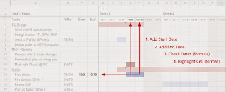
Objective: I am building project management spreadsheet like MS Project for tiny house projects, and wish to use changes in date fields to alter colors in a Gantt chart view to indicate task priority and date handling.

Status: Currently, a few columns on the left include tasks and staff assignments, as well as start and end dates. We use the right side of the sheet for a Gantt chart display, with a column for each date in the project life cycle. Conditional formatting changes the cell color for each date in which a "t" is included as a task date. This changes the cell color from the default (white) to a color indicating a date range for task handling (the character "t" and background are changed to same light red). This creates the Gantt chart view.

Sample: Below is a sample of the existing spreadsheet:

(open full-size image)

Process: To simplify management, I'd like for values in Start Date and End Date to automatically change corresponding cell colors in the Gantt chart. In Excel, I've accomplished this using a logical test in each Gantt chart cell to:

1. Get it's date from the timeline at the top of the chart, then
2. Check for "true" to test that the cell's date is "greater than or equal to" the Start Date field, and
3. Check that the cell's date is also "less than or equal to" the End Date field. 

If the above test is true (maybe AND formula?), I figure I can post a character ("t" for general tasks, though others are used to indicate task priority) in the cell which enacts automatic Conditional Formatting to create a colored cell. 

Any help with a simple and scalable solution is greatly appreciated. Thanks!

Thom Stanton

TimberTrails.TV

Timber Trails provides an empty canvass for tiny house builders via efficient, affordable, and easy-to-assemble modular SIP shells with field-friendly how-to media and support materials for building pros and DIY homeowners. Our affordable Fast-Track Design Services utilize an "adaptive design" process that slims down your favorite styles to smaller sizes while retaining real-life practicality. Turn-key customers leverage the advantage of building with SIPs, including their manufactured quality, ease of DIY construction, and incredible energy efficiency. Through a global distribution network, customers can purchase Ready-to-Raise kits, Rolling Models, and Custom Creations. All finish work is completed by independent homeowners and building trade professionals as time and budget allow. Got any other questions or want to get started on your design in a way that’s fast and affordable? Contact us to start building your one-of-a-kind tiny house, mobile cabin, or cozy cottage today. Live Large -- Go Tiny! > >  TimberTrails.TV

yogi_For Specified Weekday Compute Dates for Current Week And Future Weeks

Google Spreadsheet   Post  #2239

Yogi Anand, D.Eng, P.E.      ANAND Enterprises LLC -- Rochester Hills MI     Sep-15-2017
question by: xboxps4

https://productforums.google.com/forum/?utm_medium=email&utm_source=ba_notification#!topic/docs/Q8fczkRIngA;context-place=mydiscussions

Working out a day/date within a week ahead all the time

Hello guys,

I'll try to explain this as best as I can.  Basically I want google sheets to calculate a date based on the upcoming friday every week.  

So for example, for me today is Tue 12th Sept, so what is the upcoming friday's date?

All google sheets needs to do is give me the upcoming friday's date, so that each time I go into that spreadsheet it should have the date.

I assume this is possible based on the TODAY() formula?

Thanks very much

yogi-Conditionally Format Rows Where Cumulative Sum Of Seats For A Team Exceed 10

Google Spreadsheet   Post  #2238

Yogi Anand, D.Eng, P.E.      ANAND Enterprises LLC -- Rochester Hills MI     Sep-13-2017
question by: Apogee Rockets

https://productforums.google.com/forum/?utm_medium=email&utm_source=ba_notification#!topic/docs/LpigBGxJ5Bo;context-place=mydiscussions

Conditional Formatting for Two Columns

Hello! I'm trying to have a conditional format setting to change the color of the row when column A has ten or more entries, and/or column D has ten or more as a numerical value. Column A is a Team number and column D is a quantity number. This is the formula I have so far, but it's not working: =countif($A:$A,A1&$D:$D, D1)>10

Basically, column A is an identifier and column D is how many that team has. A Team can have multiple rows but can have no more than ten combined. So one row might have Team #1 and quantity of 7, another row has Team #1 again, and quantity of 3, equalling to ten. This is when both rows should highlight.

Thank you for any suggestions!

Screen Shot 2017-09-11 at 4.35.36 PM.png

12 KB

yogi_Pull Multiple Results For Specified Entities And Present As A Table

Google Spreadsheet   Post  #2237

Yogi Anand, D.Eng, P.E.      ANAND Enterprises LLC -- Rochester Hills MI     Sep-05-2017
question by: marklawler.za

https://productforums.google.com/forum/?utm_medium=email&utm_source=best_answer_notification_button#!topic/docs/E2dHDjQIpP8;context-place=forum/docs

Looking for help with a Sheets formula

Hi.

I'm a real novice at Google Sheets formulas and always find myself needing one that's way beyond what I know so I'm hoping someone can help me with this ...

I have 2 columns where column B has numbers that repeat randomly and column C that has random numbers that occur only once.

I want to transpose a list of column C's numbers against column B's numbers which, in the "answer array" are listed only once each.

I'm suspecting the solution will include a combination of "vlookup" and "transpose" but I haven't been able to find a solution online yet or work it out myself.

You can look at an example of what I'm trying to do HERE.

Thanks in advance ...

M a r k

yogi_Count Number Of Cases Started By Specified Shift Times

Google Spreadsheet   Post  #2236

Yogi Anand, D.Eng, P.E.      ANAND Enterprises LLC -- Rochester Hills MI     Sep-04-2017
question by: BenGenAnes

https://productforums.google.com/forum/?utm_medium=email&utm_source=best_answer_notification_button#!topic/docs/_orgPl_Us7A;context-place=forum/docs

Counting the number of cases in a specific time period

Hello all !  I have a database that tracks different operative cases in 3 different shifts in a day.  The shifts start at 7am to 3pm, then 3pm to 11pm then 11pm to 7am the following day.  We record the case, start of the operation and end of the operation in google sheets.  I've been trying to automatically count the number of cases between these shifts to give us an idea of how our hospital is performing.  I tried the formula : =COUNT(FILTER(BH2:BH, BH2:BH >= TIME(7,0,0), BI3:BI < TIME(15,0,0))), substituting the time for the 3 shifts but the total of the number of cases between the shifts does not tally to the total number of cases. Am I doing something wrong ? Help please !

Example:

Column BG Column BH Column BI

Case Start Time End Time

Appendectomy 9:23:00 10:00:00

LSCS 10:55:23 11:31:31

Appendectomy 12:21:30 12:55:00

LSCS 3:10:23 3:45:45

Appendectomy 5:30:25 6:31:31

LSCS 23:50:50 00:23:30