Friday, June 9, 2017

yogi_Pull Name From A2:A51 For Specified Debate Type In E2:E51

Google Spreadsheet   Post  #2179
Yogi Anand, D.Eng, P.E.      ANAND Enterprises LLC -- Rochester Hills MI     www.energyefficientbuild.com.   Jun-09-2017
question by Jon Baney:
https://productforums.google.com/forum/?utm_medium=email&utm_source=ba_notification#!topic/docs/LkhrFcDZ4_Y;context-place=forum/docshttps://productforums.google.com/forum/?utm_medium=email&utm_source=ba_notification#!topic/docs/8QCT_s7s_pg;context-place=mydiscussions

IF or Lookup function (If false, find next true cell)

Okay, here it goes. This is as much as I can get you, it isn't the actual sheet that I will be using, but a copy (I'm a teacher and for one, I cannot just publish student info like emails to the web, and for two...this is something that I'm creating now and won't have real data for until schools starts, so the data is fake, but it is realistic to what I need):


I have a line inserted between row 52 and 53 which divides the "tables". The lower table is based on responses in the top table (I am trying to get lists of student names who are competing in each event). I typed into each cell on row 54 what the function for that column from that point down should be looking for. To demonstrate what the data should look like as a finished product, I manually input what the table should look like after the formula is applied to each column. This "desired data" starts on the next row, 55, and continues down until in each column until there is no more "true" responses to the function.

I think I provided you with what you requested. As far as the logic goes for why I need this, I need to be able to be able to view all of the input from the top table as-is (it is actually a query pulled from another sheet that will be linked to a google form and will update as students "sign up" for each tournament) because I need to be able to view that data exclusive to that student for various reasons. I need the bottom table because I need to be able to easily see how many students are competing in all of the events without having to a) reorder the sheet or b) pull all of the responses to show and have 50+ responses under each event some of which says "student name from column A" and the rest saying "false". Starting on row 100 I have an example of what I WAS able to get, but you will see why that is undesirable...I want each column to only show the "true" responses--though, in collumn 101D-101L, I am not sure how to make those formulas search for a phrase within text and kick back a true statement if true, which is what I want (and is my second question listed in my original post). Example desired formula: Give me the value for column A any time column F contains "informative speaking":

Cell F="Informative Speaking, Original Oratory" (THE FORMULA IS TRUE!)
Cell F="Informative Speaking" (THE FORMULA IS TRUE!)
Cell F="Original Oratory, International Extemp" (THE FORMULA IS FALSE; this cell would show the next true statement.)
Cell F="International Extemp, Informative Speaking" (THE FORMULA IS TRUE; this would actually appear in the cell above because it was false)

I hope I am explaining this all correct and that it can all be done. 

Thanks for your help!


yogi_Mark Names Of Actors That Are Out Based On Form Submittals Of Date Out And Date Back

Google Spreadsheet   Post  #2178
Yogi Anand, D.Eng, P.E.      ANAND Enterprises LLC -- Rochester Hills MI     www.energyefficientbuild.com.   Jun-07-2017
question by SMintheHat:
https://productforums.google.com/forum/?utm_medium=email&utm_source=ba_notification#!topic/docs/LkhrFcDZ4_Y;context-place=forum/docs
Vlookup not searching through duplicates
Hello all!

I've gotten a lot of advice from this forum and have created the following sheet to help with work:

In short it is a way to tell which actor is out based on data entered in the form linked to the sheet and the date at the top of the sheet.
The main search formula is:

=iferror(if(and(vlookup(A4,'Actors Out'!$A$2:$A,1,0),$B$1>=index('Actors Out'!$B$2:$B,match(A4,'Actors Out'!$A$2:$A,0)),$B$1<index('Actors Out'!$C$2:$C,match(A4,'Actors Out'!$A$2:$A,0))),"OUT",""),"")

The problem I'm having is that vlookup is stopping at the first actors name which shows up in the Actors Out form. When there is someone with multiple days out(Example AMY) "OUT" will show up as out when B1 is between 5/30/17 and 6/1/17 but not when B1 is between 6/8/17 and 6/10/17.

Please let me know if there is another to find if the actor will be out based on the cell B1 and the information being entered into the google form.

Thank you!


Wednesday, June 7, 2017

yogi_Conditionally Format Entire Row Where The SearchBox Item is Found Any Where In The Corresponding Row

Google Spreadsheet   Post  #2177
Yogi Anand, D.Eng, P.E.      ANAND Enterprises LLC -- Rochester Hills MI     www.energyefficientbuild.com.   Jun-07-2017
question by Thomas KM:
https://productforums.google.com/forum/?utm_medium=email&utm_source=ba_notification#!topic/docs/-gIkDcJbil8;context-place=forum/docs
How do I create a function to highlight cells that contain text specified in a search cell
Hello,
I was wondering if you might be able to help me with an issue I'm facing creating a search/highlight cell in a spreadsheet. I'm looking to be able to type a word into a box at the top of my sheet and then have every row where this word occurs highlighted in the sheet below. I see that there are a few ways to do this in Excel, but I haven't been able to do this here. 
Thank you,
Thomas

Here is a link to the sheet I've been working on:
https://docs.google.com/spreadsheets/d/1N3hZqcradkbm7Y7MAED73nDHT_yXkSSettkctjj3_Rc/edit?usp=sharing
Here is a link to the kind of thing I'm looking for:
https://exceljet.net/tips/how-to-build-a-search-box-to-highlight-data


yogi_WorkAround for Query() - Creating New Column by combining Year & Month

Google Spreadsheet   Post  #2176
Yogi Anand, D.Eng, P.E.      ANAND Enterprises LLC -- Rochester Hills MI     www.energyefficientbuild.com.   Jun-07-2017
question by KW LowTS:
https://productforums.google.com/forum/?utm_medium=email&utm_source=ba_notification#!topic/docs/fTNDCXkP0yg;context-place=forum/docs
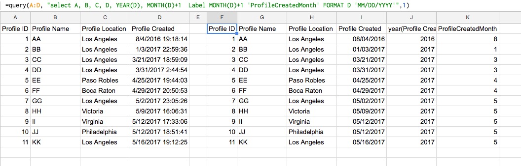
Query() - Creating New Column by combining Year & Month

I have a query that returns the expected results
=query(A:D, "select A, B, C, D, YEAR(D), MONTH(D)+1 Label MONTH(D)+1 'ProfileCreatedMonth' FORMAT D 'MM/DD/YYYY'",1)

But, I'm trying to create a new column that is the combination of YEAR(D) & MONTH(D)+1 ie "2017-05" or "2016-12". Since query() does not allow merging columns and because dates are more complex to work with, can any recommend a workaround?

[Edited]Or even if there's a way to show a 2nd occurrence of D where I can FORMAT the 2nd occurrence of D to be 'YYYY-MM'. I need the 1st occurrence of D.

Thanks


Monday, June 5, 2017

yogi_Compute Row By Row Sum For Rows 1 to 12 Of Scores From A Number Of Columns

Google Spreadsheet   Post  #2175
Yogi Anand, D.Eng, P.E.      ANAND Enterprises LLC -- Rochester Hills MI     www.energyefficientbuild.com.   Jun-05-2017
question by Tyler_Zhu:
https://productforums.google.com/forum/?utm_medium=email&utm_source=ba_notification#!topic/docs/bx4wShnjOec;context-place=mydiscussions
Sheets: Repeat the same function on the values in a row for many rows
I have found that very often, I wish to do the same basic operation on many rows in Google Sheets. For example, I used to have a contest logger of which questions I got right when doing practice contests, and at the end of each row I would sum over all the points that I got right in that row. I would then repeat this for each new contest, a.k.a. each new row. See attached picture and ignore all of the color coding. 

More recently, I have just finished administering a contest and I want to keep the scores in a Google Sheets. The rows would be the different contestants, and I want to keep track of which questions they get right or wrong, with a total of their points at the end, much like how I set up my tracker in the attached picture. However, I do not wish to have to do " =SUM(D15:AB15) " 100 times to get the sum. Is there any simple way of repeating this operation for many rows?

Sunday, June 4, 2017

yogi_Remove 'as of date and space character' from entries in column A In-Situ

Google Spreadsheet   Post  #2174
Yogi Anand, D.Eng, P.E.      ANAND Enterprises LLC -- Rochester Hills MI     www.energyefficientbuild.com.   Jun-04-2017
question by Kathy VanDeven:
https://productforums.google.com/forum/?utm_medium=email&utm_source=ba_notification#!topic/docs/ATVtdBVqt_A;context-place=mydiscussions
How do I replace text and date with nothing?
as of 02/28/2017 PIMCO INCOME FUND CL D
as of 03/28/2017 VANGUARD WELLINGTON INVESTOR
as of 03/28/2017 VANGUARD/WELLESLEY INCOME INVESTOR
as of 03/31/2017 HENNESSY GAS UTILITY INVESTOR CL

want to replace as of and whatever date that follows it.  I am using a Chromebook. 

yogi_Round Entries (greater than or less than 1) To Nearest Specified Number

Google Spreadsheet   Post  #2173
Yogi Anand, D.Eng, P.E.      ANAND Enterprises LLC -- Rochester Hills MI     www.energyefficientbuild.com.   Jun-04-2017
question by SolveAllProblemsRightNow:
https://productforums.google.com/forum/?utm_medium=email&utm_source=ba_notification#!topic/docs/rO5IdnrVgz0;context-place=forum/docs
[ g-excel ] -- rounding to the nearest 5 -- chrome extension, functions, etc.

6 > 5
.7 > .5
13 > 15
.022 > .020
1368 > 1370
that's what call rounding to the nearest 5, 10, 15, 20...
* what function or chrome extension or any solution that can do this?
* can excel do this?

---
see unsolved here -> https://paper.dropbox.com/doc/2015-2025-THE-FUCKING-HELL-OF-GOOGLE-SOFTWARE-HOLY-SHIT-LIST-OF-G-PROBLEMS-6TYv5Ye144H2PQY4HhQLM