yogi_Conditionally Format Range S3:DY7 For Production Days For Each Install

Google Spreadsheet   Post  #2240

Yogi Anand, D.Eng, P.E.      ANAND Enterprises LLC -- Rochester Hills MI     Sep-17-2017
(Comment by Jeremy Knightly )to original question by: ThomFlash 

How to automate Gantt Chart creation using logical expressions to change cell colors...

Objective: I am building project management spreadsheet like MS Project for tiny house projects, and wish to use changes in date fields to alter colors in a Gantt chart view to indicate task priority and date handling.

Status: Currently, a few columns on the left include tasks and staff assignments, as well as start and end dates. We use the right side of the sheet for a Gantt chart display, with a column for each date in the project life cycle. Conditional formatting changes the cell color for each date in which a "t" is included as a task date. This changes the cell color from the default (white) to a color indicating a date range for task handling (the character "t" and background are changed to same light red). This creates the Gantt chart view.

Sample: Below is a sample of the existing spreadsheet:

(open full-size image)

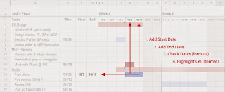
Process: To simplify management, I'd like for values in Start Date and End Date to automatically change corresponding cell colors in the Gantt chart. In Excel, I've accomplished this using a logical test in each Gantt chart cell to:

1. Get it's date from the timeline at the top of the chart, then
2. Check for "true" to test that the cell's date is "greater than or equal to" the Start Date field, and
3. Check that the cell's date is also "less than or equal to" the End Date field. 

If the above test is true (maybe AND formula?), I figure I can post a character ("t" for general tasks, though others are used to indicate task priority) in the cell which enacts automatic Conditional Formatting to create a colored cell. 

Any help with a simple and scalable solution is greatly appreciated. Thanks!

Thom Stanton

TimberTrails.TV

Timber Trails provides an empty canvass for tiny house builders via efficient, affordable, and easy-to-assemble modular SIP shells with field-friendly how-to media and support materials for building pros and DIY homeowners. Our affordable Fast-Track Design Services utilize an "adaptive design" process that slims down your favorite styles to smaller sizes while retaining real-life practicality. Turn-key customers leverage the advantage of building with SIPs, including their manufactured quality, ease of DIY construction, and incredible energy efficiency. Through a global distribution network, customers can purchase Ready-to-Raise kits, Rolling Models, and Custom Creations. All finish work is completed by independent homeowners and building trade professionals as time and budget allow. Got any other questions or want to get started on your design in a way that’s fast and affordable? Contact us to start building your one-of-a-kind tiny house, mobile cabin, or cozy cottage today. Live Large -- Go Tiny! > >  TimberTrails.TV

yogi_For Specified Weekday Compute Dates for Current Week And Future Weeks

Google Spreadsheet   Post  #2239

Yogi Anand, D.Eng, P.E.      ANAND Enterprises LLC -- Rochester Hills MI     Sep-15-2017
question by: xboxps4

https://productforums.google.com/forum/?utm_medium=email&utm_source=ba_notification#!topic/docs/Q8fczkRIngA;context-place=mydiscussions

Working out a day/date within a week ahead all the time

Hello guys,

I'll try to explain this as best as I can.  Basically I want google sheets to calculate a date based on the upcoming friday every week.  

So for example, for me today is Tue 12th Sept, so what is the upcoming friday's date?

All google sheets needs to do is give me the upcoming friday's date, so that each time I go into that spreadsheet it should have the date.

I assume this is possible based on the TODAY() formula?

Thanks very much

yogi-Conditionally Format Rows Where Cumulative Sum Of Seats For A Team Exceed 10

Google Spreadsheet   Post  #2238

Yogi Anand, D.Eng, P.E.      ANAND Enterprises LLC -- Rochester Hills MI     Sep-13-2017
question by: Apogee Rockets

https://productforums.google.com/forum/?utm_medium=email&utm_source=ba_notification#!topic/docs/LpigBGxJ5Bo;context-place=mydiscussions

Conditional Formatting for Two Columns

Hello! I'm trying to have a conditional format setting to change the color of the row when column A has ten or more entries, and/or column D has ten or more as a numerical value. Column A is a Team number and column D is a quantity number. This is the formula I have so far, but it's not working: =countif($A:$A,A1&$D:$D, D1)>10

Basically, column A is an identifier and column D is how many that team has. A Team can have multiple rows but can have no more than ten combined. So one row might have Team #1 and quantity of 7, another row has Team #1 again, and quantity of 3, equalling to ten. This is when both rows should highlight.

Thank you for any suggestions!

Screen Shot 2017-09-11 at 4.35.36 PM.png

12 KB

yogi_Pull Multiple Results For Specified Entities And Present As A Table

Google Spreadsheet   Post  #2237

Yogi Anand, D.Eng, P.E.      ANAND Enterprises LLC -- Rochester Hills MI     Sep-05-2017
question by: marklawler.za

https://productforums.google.com/forum/?utm_medium=email&utm_source=best_answer_notification_button#!topic/docs/E2dHDjQIpP8;context-place=forum/docs

Looking for help with a Sheets formula

Hi.

I'm a real novice at Google Sheets formulas and always find myself needing one that's way beyond what I know so I'm hoping someone can help me with this ...

I have 2 columns where column B has numbers that repeat randomly and column C that has random numbers that occur only once.

I want to transpose a list of column C's numbers against column B's numbers which, in the "answer array" are listed only once each.

I'm suspecting the solution will include a combination of "vlookup" and "transpose" but I haven't been able to find a solution online yet or work it out myself.

You can look at an example of what I'm trying to do HERE.

Thanks in advance ...

M a r k

yogi_Count Number Of Cases Started By Specified Shift Times

Google Spreadsheet   Post  #2236

Yogi Anand, D.Eng, P.E.      ANAND Enterprises LLC -- Rochester Hills MI     Sep-04-2017
question by: BenGenAnes

https://productforums.google.com/forum/?utm_medium=email&utm_source=best_answer_notification_button#!topic/docs/_orgPl_Us7A;context-place=forum/docs

Counting the number of cases in a specific time period

Hello all !  I have a database that tracks different operative cases in 3 different shifts in a day.  The shifts start at 7am to 3pm, then 3pm to 11pm then 11pm to 7am the following day.  We record the case, start of the operation and end of the operation in google sheets.  I've been trying to automatically count the number of cases between these shifts to give us an idea of how our hospital is performing.  I tried the formula : =COUNT(FILTER(BH2:BH, BH2:BH >= TIME(7,0,0), BI3:BI < TIME(15,0,0))), substituting the time for the 3 shifts but the total of the number of cases between the shifts does not tally to the total number of cases. Am I doing something wrong ? Help please !

Example:

Column BG Column BH Column BI

Case Start Time End Time

Appendectomy 9:23:00 10:00:00

LSCS 10:55:23 11:31:31

Appendectomy 12:21:30 12:55:00

LSCS 3:10:23 3:45:45

Appendectomy 5:30:25 6:31:31

LSCS 23:50:50 00:23:30

yogi_Pull Category From List Of Transactions Based On 'Place Of Business'

Google Spreadsheet   Post  #2235

Yogi Anand, D.Eng, P.E.      ANAND Enterprises LLC -- Rochester Hills MI     Sep-01-2017
question in: mpuchtel

https://productforums.google.com/forum/?utm_medium=email&utm_source=footer#!topic/docs/zu_2vuOk41Y;context-place=forum/docs

Coders looking for a challenge? I need to create a custom labeling function!!!

 Hello,

I have a list of bank transactions that include various transaction descriptions. I want to write an arrayed function that will search each description, seek out any key words such as "starbucks", and output a type such as "eating out". I figure this is somehow possible if I create a table that defines the relationship between key words and output types, but I'm not sure how to write a function that searches the table and gives me the output I desire. 

Any feedback is appreciated - thanks!!

Max

yogi_Conditionally Format -- Highlight Names That Meet Specified Criteria (noted in cells F26:G28)

Google Spreadsheet   Post  #2234

Yogi Anand, D.Eng, P.E.      ANAND Enterprises LLC -- Rochester Hills MI     Aug-31-2017
question in: Whitney Andersen

https://productforums.google.com/forum/?utm_medium=email&utm_source=footer#!topic/docs/QQbNLslmQlQ;context-place=forum/docs

Data validation
I have a doc with a series of Data Validations and I wanted to have a cell be flagged if another cell has a certain drop down entered unless a drop down in another cell is checked. Ill share the sheet and I wrote the explination of what im trying to do in Cells F26 - G26, and F28-G28

https://docs.google.com/spreadsheets/d/10HJ9_pGL9a823Xi2fGTOdO-1eeOnPqt0OmpXRTft2NY/edit?usp=sharing

yogi_Going Row Wise Conditionally Format -- Highlight Subsequent Instances Of Names That Have Already Occurred

Google Spreadsheet   Post  #2233

Yogi Anand, D.Eng, P.E.      ANAND Enterprises LLC -- Rochester Hills MI     Aug-29-2017
question in: TCs Friendly Circle

https://docs.google.com/spreadsheets/d/17zzR1I1FWLxeL8LGLSTGfl9kS-tRKVBwn50YHYIaIUs/edit?usp=sharing

Going Row Wise Conditionally Format -- Highlight Subsequent Instances Of Names That Have Already Occurred

yogi_Conditionally Format (Highlight Duplicate Entries In Column A While Ignoring * Character In The Entry

Google Spreadsheet   Post  #2231

Yogi Anand, D.Eng, P.E.      ANAND Enterprises LLC -- Rochester Hills MI     Aug-27-2017
question by: Paulo Miguel

https://productforums.google.com/forum/?utm_medium=email&utm_source=footer#!msg/docs/6bODIHZwWbg/syOPinS7CAAJ

Issue with asterisks and conditional formatting

I have the following in column A:

12345

12345*

1234567*890

And the following in conditional formatting:

=countif(A:A,A:A)>1

The issue is that 12345* gets marked when it obviously shouldn't be. After a bit of testing I found out it was the asterisk likely messing up with the formula, since 12345* does match with 1234567*890 if wildcards were active (which they are), just like 1234567*890 would be marked if something like 1234567XXXXX890 was in the column.

So my question is if there's any way to either disable wildcards for this formula or if there's any way around this issue.

Any help would be appreciated.

yogi_Conditionally Format 'Ingredients To Avoid' That Are In 'Ingredients List'

Google Spreadsheet   Post  #2230

Yogi Anand, D.Eng, P.E.      ANAND Enterprises LLC -- Rochester Hills MI     Aug-26-2017
question by: jorasdou

https://productforums.google.com/forum/?utm_medium=email&utm_source=best_answer_notification_button#!topic/docs/xUn8Kb5GZvs;context-place=forum/docs

Possible to enter a list of items in one cell and have matches in other cells highlight?

 

Apologies in advance, because I'm not tech- or formula-savvy. I have a skin condition that requires me to be avoid certain ingredients; I can usually remember most of them, but sometimes it's hard to remember all of them. While I'm shopping for products online (because I'm still trying to find things that help), I'm having to read through ingredient lists to look for problematic items, usually multiple times in order to check for each thing.

I'm wondering if there's a way to set up a Sheet and formula for this:

-Ingredients To Avoid are already listed in individual cells

-I copy/paste a product's full ingredients list into a specific cell (a large merged cell)

-Any word matches between the two lists would result in that ingredient's cell being highlighted on the Ingredients To Avoid list

I set this up for example -- the full list of ingredients has Alcohol Denat, Castor Oil, and Fragrance, so three cells are colored in:

The Ingredients To Avoid list isn't complete, so I'd need to know how to change the formula to incorporate the additional items. But is this even possible? Or will it not work due to the product's full list of ingredients not being listed in individual cells?

yogi_Compute Row By Row Running Total Of Value By Type Where Date is Less Than Or Equal To Date In Current Row

Google Spreadsheet   Post  #2229

Yogi Anand, D.Eng, P.E.      ANAND Enterprises LLC -- Rochester Hills MI     Aug-20-2017
question by: Henrique Magalhaes

https://productforums.google.com/forum/?utm_medium=email&utm_source=ba_notification#!topic/docs/1cjhkWHcKC4;context-place=forum/docs

Array formula with sumif with less than condition

Hi, I have this sheet with the following columns of data:

Column A - Date: this is the date of a transaction.

Column B - Type: this is the type of the item

Column C- Value: this is the value of the transaction

For each row, I need to determine 2 values:

Column D. the sum of all values of the current type, where date is equal the current date. I've used the following formula to achieve that: sumifs(C:C;A:A;A2;B:B;B2).

Column E. the sum of all values of the current type, where date is less than or equal the current date. I've used the following formula to achieve that: sumifs(C:C;A:A;"<="&A2;B:B;B2).

However this sheet will be used with a great amount of data, and I need it to auto populate new rows with these formulas. Arrayformula does that well for the first one, and I changed it to: =arrayformula(if(row(A:A)=1;"sum of type in current date";sumif(A:A&B:B;A:A&B:B;C:C))).  Sumifs didn't work so I changed it to a formula with sumif and & operators.

However I could not think how to make it for the column E formula. Is there any way to use arrayformula with sumif (or sumifs) and "<=" condition? If not, is there any other way to auto populate the formula to new lines?

Thanks

yogi_Compute Running Total Of Value By Type Where Date is Less Than Or Equal To Today's Date

Google Spreadsheet   Post  #2228

Yogi Anand, D.Eng, P.E.      ANAND Enterprises LLC -- Rochester Hills MI     Aug-20-2017
question by: Henrique Magalhaes

https://productforums.google.com/forum/?utm_medium=email&utm_source=ba_notification#!topic/docs/1cjhkWHcKC4;context-place=forum/docs

Array formula with sumif with less than condition

Hi, I have this sheet with the following columns of data:

Column A - Date: this is the date of a transaction.

Column B - Type: this is the type of the item

Column C- Value: this is the value of the transaction

For each row, I need to determine 2 values:

Column D. the sum of all values of the current type, where date is equal the current date. I've used the following formula to achieve that: sumifs(C:C;A:A;A2;B:B;B2).

Column E. the sum of all values of the current type, where date is less than or equal the current date. I've used the following formula to achieve that: sumifs(C:C;A:A;"<="&A2;B:B;B2).

However this sheet will be used with a great amount of data, and I need it to auto populate new rows with these formulas. Arrayformula does that well for the first one, and I changed it to: =arrayformula(if(row(A:A)=1;"sum of type in current date";sumif(A:A&B:B;A:A&B:B;C:C))).  Sumifs didn't work so I changed it to a formula with sumif and & operators.

However I could not think how to make it for the column E formula. Is there any way to use arrayformula with sumif (or sumifs) and "<=" condition? If not, is there any other way to auto populate the formula to new lines?

Thanks