yogi_Insert Special Characters Such As € And £ In Spreadsheet

Yogi Anand, D.Eng, P.E.                                         Google Spreadsheet                            www.energyefficientbuild.com

estupido said:
how do I insert special characters into a google docs spreadsheet. For example the symbol for the euro or pound.
-----------------------------------------------------------
On an Amrican keyboard there are no keys for characters such as € and £ ... so one has to resort to special key combinations / codes to make entries for such special characters.
In the following I have used special characters such as the € and the £ in TEXT as well as in FORMULAS

yogi_Sum Up Numbers In A Column Corresponding To Non-Blank Rows In Another Column

Yogi Anand, D.Eng, P.E.                                         Google Spreadsheet                            www.energyefficientbuild.com

anandrajk said:
Use the SUM IF function to add only those cells corresponding to a non-empty cell in the specified range.
for eg. in column C i have values ( numbers, text and empty cells). I want to add all the cells in column D that have non-empty cells in column C.
I know how to search for blank cells and it works. I use SUMIF(C3:C10,"",D3:D10) . This sums all values in column D for which column C is blank. I want to do the opposite.
would appreciate any help
----------------------------------------------------------------
In the following ...
I have a solution using SUMIF function in Sheet1
a solution using the FILTER function in Sheet2
Sheet3 has a solution using the QUERY function (by first convering all entries in range C:D to TEXT)
Sheet4 has another solution using the QUERY function and aggregating column D
by the way in this case solutions using the SUMIF and the FILTER function are so straight forward
I have included the solution using the QUERY function out of interest especially since column C is mixed TEXT, NUMBERS, and BLANKS

yogi_Substitute Part Of A String With A Variable In ImportXML Formula

Yogi Anand, D.Eng, P.E.                                         Google Spreadsheet                            www.energyefficientbuild.com

Amoner said:
Substituting a part of the formula with the content of an adjacent cell
I am trying to modify my [code]=importXML("http://www.google.com/search?q=B1&num=100", "//a[@class='l']/@href")[/code] and "B1" is where formula should grab the content from... I have tried a multiple number of ways to fix the problem. But what I would want is that I modify the B1 cell and it refreshes the formula. Trying to simplify the process for my co-workers. Is this doable?


Updates:
ignore [code] part
So the 2nd column is what the result should be like, but if you try substituting "Swiss Colony" with B1, it just searches for B1. Which makes sense because it all enclosed in "" , so I tried breaking it down into separate parts to make B1 an active element, I succeeded with that in D2 and the following. But it wont execute it, because google reads is an an outcome not an input...
------------------------------------------------------------------------------
ImportXML formula in cell B2 uses the string Swiss Colony
I have created a formula in cell C2 which uses the variable in cell B1 instead of the literal string Swiss Colony

yogi_Chart, Image, Formatted Text, And Hyperlink In Blog Post

Yogi Anand, D.Eng, P.E.                                  Google Spreadsheet                     www.energyefficientbuild.com

yogi_Compute Y The Number Of Occurrences Of X In A Specified Column

Yogi Anand, D.Eng, P.E.                                         Google Spreadsheet                            www.energyefficientbuild.com

F.R.S. said:
It would be cool, if anybody can help me here. Unfortunately, I didn't find anything on the web so far :(
I have a table and in column D, I want to store multiple numbers as a comma separated list, e.g.:
D
03
04,10
10
05,07
10,12
etc.
In another sheet, I want to count how many cells contain a certain number. What I did so far is:
=COUNT(FILTER(Sheet1!D:D,SEARCH(10,Sheet1!D:D)))
If D is formated as numbers and only use one number (instead of a list) in every D-cell, this works fine.
On the other hand, the formula does not work anymore for comma separated list that is formated as text.
Interestingly, also single numbers don't work if they are formated as text.
------------------------------------------------------------------------
In the following solution I have computed Y for occurrence of X with different solutions in
Sheet1, Sheet2, and Sheet3

yogi_Get Closing Price For Multiple Stocks For A Given Date

Yogi Anand, D.Eng, P.E.                                         Google Spreadsheet                            www.energyefficientbuild.com

chandan.ssj said:
how can i get closing price for multiple stocks for a given date?
i am new to google finance spreadsheet.
I'd like to create a data table that holds the historical prices of a list of stocks, getting the closing price for each stock for a given date.
So, say A2 - A7 holds the following:
DELL
MO
PG
JNJ
CSCO
XOM
and cell B1 holds 2/2/2011
What I'm trying to acheive is generating a table like this:
A B
2/2/2011
2 DELL 158
3 MO 49
4 PG 241
5 JNJ 12
6 CSCO 741
7 XOM 54
------------------------------------------------------------------
I don't know about where you got the numbers in your column B from
I have provided a formula in cell B2 that is then dragged down for copying as far as needed


----------------------------------------------------------------
chandan.ssj further added:
now in the same spreadsheet if I wanted to add few more attributes, (for example open price), in column C, then what will be the formula used?
I have added Sheet2 where I have setup the formula for close and open prices ... in fact you can extend it for other GoogleFinance function attributes as well.

yogi_Get Header Name Of Column(s) Containing Data That Matches A Specified Value

Yogi Anand, D.Eng, P.E.                                         Google Spreadsheet                            www.energyefficientbuild.com

edanishafridi said:
How do i get the header name of columns containing data which matches my query?
example
    A      B      C
1 group1 group2 group3
2 21 25 26
3 56 12 3
4 98 45 16
QUERY= 12
which formula do i use to get the header name of the column containing 12 i.e. in the above case group2.
i have search alot but didn't find the axact what i am looking for.
-------------------------------------------------------------------------------

yogi_Extract The Row(s) That Occur Most Often Based On Data In Columns A And B

Yogi Anand, D.Eng, P.E.                                         Google Spreadsheet                            www.energyefficientbuild.com

crook_ed said:
I have to columns of data, Column A and column B. I want to count the data in column B based on the data in column A. Once i have the count, i have to produce row which appears the most.
For example, Column A consist of Items codes, and Column B consist of company names.
Item codes Company Names
1001 A
1001 A
1001 A
1001 B
1001 B
1002 A
1002 A
1002 B
1002 B
1002 B
My result should be the same as shown below, because both pairs appear the most number of times.
1001 A
1002 B
-----------------------------------------------------------------------------------
In Sheet1 the solution outputs the result in two columns with a geralized solution using ranges A:A, and B:B
and
in Sheet2 the solution outputs the result in one column using ranges A2:A11, and B2:B11

yogi_Count Number Of Times A Specific Value Is In A And B Has A Certain Value In Corresponding Row

Yogi Anand, D.Eng, P.E.                                         Google Spreadsheet                            www.energyefficientbuild.com

prolink007 said:
I am having trouble righting a function for this need (in google spreadsheets):
I have 2 columns A and B.
I want to be able to get a percentage based on those two columns. I want to count the number of times a specific value is found in A and only if B has a certain value in it.
Example:
A contains the following values name1, name2, name7, name1, name1, name2
B contains the following values yes, no, no, yes, no, yes (with respect to column A)
I would like to function to only give me the percentage of times name1 is found when it is associated with a yes in column B.
---------------------------------------------------------------------------

in the following I have a formula in cell D2 for count of yes entries for a single name
and
in celle E2, and F2, I have formulads for yes entries for all the names in column A

yogi_Calculate A Date X Days From A Fixed Date Skipping Sundays

Yogi Anand, D.Eng, P.E.                                         Google Spreadsheet                            www.energyefficientbuild.com

maggyk said:
I'm designing a spreadsheet that records employee work hours. Pay periods run from the 2nd business day prior to the 1st and 16th of the month through the 3rd business day prior to the 1st/16th. (e.g., the first pay period of this month started on Wednesday, April 27th and ended on the Wednesday, May 11th. The last pay period of this month started on Thursday, May 12th and ended on Thursday, May 26th.) I was soooo close setting up reference cells in column A of 1/1/11, 1/16/11, 2/1/11, etc., and then calculating the end of a pay period in Column C with =workday(A2,-3) and the beginning of the next pay period in Column B (next row) with =workday(C2,1). Unfortunately, it turns out this organization works on Saturdays, so I need to be able to return a value if it falls on a Saturday, but skip Sundays and return the date of the following Monday. Any suggestions for a calculation that will help?
--------------------------------------------------------------------------------
here we go maggyk ... have a look at the following solution and see if this would do.

yogi_Calculate Gestational Age Of Pregnancy In Fractional Weeks

Yogi Anand, D.Eng, P.E.                                         Google Spreadsheet                            www.energyefficientbuild.com

jgoodw said:
I have the formula that works in regular Excel but when I use this formula in Google Docs the fraction that I want to report as #/7 instead lists as a fraction.
The formula that works in Excel is:
=IF(U8=ʺʺ,ʺʺ,((40-((U8-(TODAY()))/7))))
Any help would be great!
Update:
I need the results to read as the gestational age would:
For example if someone is 34weeks and 6 days I want it to show as 34 6/7; I would also be ok with 34 6. The formula listed instead gives me a decimal which doesn't work because someone can't be 34weeks a .9 days.
----------------------------------------------------------------------------

yogi_Reinstate Deleted Form In Google Spreadsheet

Yogi Anand, D.Eng, P.E.                                         Google Spreadsheet                            www.energyefficientbuild.com

keithx8 said:
It appears that the "Form" function in Google Docs creates a spreadsheet.  It appears that the process cannot operate in the reverse - in other words, if I create a spreadsheet, I don't see how it can be converted to a form.

Since I accidentally deleted my form, I am left with the spreadsheet, which doesn't help me - I need the form for others to enter data.

Operating System:  MS Windows 7 Home Premium; Browser:  Chrome

--------------------------------------------------------------------------------

In the following I have used a simple 6 step process to reinstate the deleted Form associated with the original ResponseTable

here is the Form that is associated with the ResponseTable of the spreadsheet

and the following is the Response summary with last two submittals having been made via Form in the Blog

yogi_Extract Entries Starting With ? From Spreadsheet Cells

Yogi Anand, D.Eng, P.E.                                         Google Spreadsheet                            www.energyefficientbuild.com

henry922 said:
For example here's a spreadsheet with texts
A B
---------
?apple banana
orange pear
mango ?melon
And my expected output:
?apple
?melon
Any ideas? I'm new to google docs...
---------------------------------------------------------------------------

yogi_Compute Sum For Vendors Sponsor Amount Where Amount Column Has Some Text Entries

Yogi Anand, D.Eng, P.E.                                   Google Spreadsheet                     www.energyefficientbuild.com

ThimoGFR said:
I have an Importation sheet with several information. In there are several different vendors with several single orders. Sometimes we get a discount or sponsoring.
What I want is a formula, which sums up the complete sponsoring of a vendor. Problem is that I get new vendors every and I do not want to type the name of the vendor. I tried it with pivot table report - there I could group vendors and with a filter I could sum the sponsoring. Here the Problem is that Pivot table does not really work for me because it destroys my whole sheet.
Sometimes in column V i have "*****" which are not numeric.
---------------------------------------------------------------------------------------

following is an image of part of the Importation sheet

Importation

yogi_Gadget Table With Filter And Grouping -- y20110521h1-01

Yogi Anand, D.Eng, P.E.                                  Google Spreadsheet                     www.energyefficientbuild.com

yogi_Calculate X Percent Of A Number Which Then Is Successively Decreased By Y Percent

Yogi Anand, D.Eng, P.E.                                         Google Spreadsheet                            www.energyefficientbuild.com

andie856603 said:
what formula do i need to calculate 75% of a number which then decreases by 90%
i also need to do with this also is add another value...yes the original number will stay the same but where would i enter the column/row to show if it was the 1st/2nd/3rd etc calcution of this number ie 1 would be 75% of original then 2 90% of that 3 90% of 2..... 4 90% of 3 and so on.

-----------------------------------------------
I believe I have answered this question from Andrea before ... in any event here we go again. I have generalized it though by using variable percentages A and B rather than the static values of 75% and 90%

yogi_Insert A Cell Value In An Import Function

Yogi Anand, D.Eng, P.E.                                         Google Spreadsheet                            www.energyefficientbuild.com

franzellin said:
I have a function where I import from yahoo finance the value of an option, the value is defined as:
=arrayformula(substitute(Index(ImportHtml("http://finance.yahoo.com/q?s=TBT110618p00035000"&"&workaround="&INT(googleclock()*1e10);"table";1);1;2);"*";""))
I would like to modify TBT110618p00035000 in
&A1&A2&A3&000&A4&000 where
a1= cell with the content "TBT"
a2= cell with the content "110618"
a3= cell with the content "c"
a4= cell with the content "35"
and
I tried to simplify
cell B18=TBT110618p00035000
cell C18=index(ImportHtml("http://finance.yahoo.com/q?s=&B18&";"table";1);1;2)
but I have still no success
-----------------------------------------------------------------------
In reference to the first question I have incorporated the values of variable entries in cells A1,A2,A3, and A4 in the formula in cell B6
and
in cell B10 the formula in cell b2 is modified to incorporate the variable entry in cell A10

yogi_Sum Of Specific Columns Based On A Pattern In Each Row

Yogi Anand, D.Eng, P.E.                                         Google Spreadsheet                            www.energyefficientbuild.com

Justin Bradley said:

I want to calculate the sum of certain columns for each row. Ex I want =SUM(F8,L8,R8,X8,AD8), then under that I want =SUM(F9,L9,R9,X9, AD9). Is there any way to automate this for each row like =SUM (F*,L*,R*,X*,AD*) where *= the row number?
----------------------------------------------------------------------------
Well, I noticed the pattern that starting with column F you want to sum up the value in every 8th column in row 8 and once a formulas has been developed do that for row 8, then the formula can be replicated for row 9.

yogi_Apply Two Filter Functions In Spreadsheet

Yogi Anand, D.Eng, P.E.                                         Google Spreadsheet                            www.energyefficientbuild.com

Pettere said:
I am trying to apply two filter functions in Google Docs.
•Column (A) contains new data
•Column (B) contains filter data, i.e. cells with text that should not be included in column C
•Column (C) is the outcome, i.e. column A minus all the cell data in column B
Example: www.goo.gl/idyXy
I use this formula in column C: =ARRAYFORMULA(SORT(UNIQUE(IF(ISNA(MATCH(A2:A,B2:B,0)),A2:A,""))))
It works well in the sense that it filters data (in this case e-mail addresses) that should not be included in column C. However, I would also like to be able to filter whole domains, i.e. if the domain example.com is listed in column B then all addresses from column A ending with example.com should be excluded from column C.

Update by Petteri:

In column A I have new e-mail addresses.

In column B I have a filter list consisting of e-mail addresses and domains.

Column C should be the result of all the e-mail addresses in column A minus the e-mail addresses in column B, however the e-mail addresses from column A which have a corresponding domain name in column B should also be excluded.

Example:

A: jimmy@itcompany.com, arne@itcompany.com, fred@webcompany.com

B: jimmy@itcompany.com, webcompany.com

C: arne@itcompany.com

Column A is the new list.

Column B is the filter list (e-mail addresses and the occasional domain)

Column C is the result, A minus B.

--------------------------------------------------------------------------------------------

yogi_Get Information From The Next Row Down Without Having To Change All Tthe Formulas One By One

Yogi Anand, D.Eng, P.E.                                         Google Spreadsheet                            www.energyefficientbuild.com

heatherd1015 said:

I have a painting company and I use a google form to gather information about the rooms my clients want painted. Every time I submit a new form the information is put into a google spreadsheet that I use to estimate job costs. I have the room measurement the clients name and address and my calculations all on sheet 1. Every column is labeled the same, the information just varies row to row.
So the first customers information gets put into row 1. The next customer is in row 2 and so on. This is sheet 1.
Sheet 2 I have as a Estimate form that I can print and give to the customer. It has my business name, the estimate # and the total job cost. Lets say I have the formula in the "name" cell on my estimate to be. =Sheet1!G16 which returns "Heather" I complete the rest of the cell formulas to pull various information from row 16. Such as Job description, total cost, etc. I print the form and I am done and now I need to print another estimate for the next client whose information is all on row 17.
Is there a way I can change all the number 16's: A16, G16, L16, to A17, G17, and L17 automatically? I don't want to have to waste my time changing the formulas every time I have to create a new estimate.

--------------------------------------------------------------------------

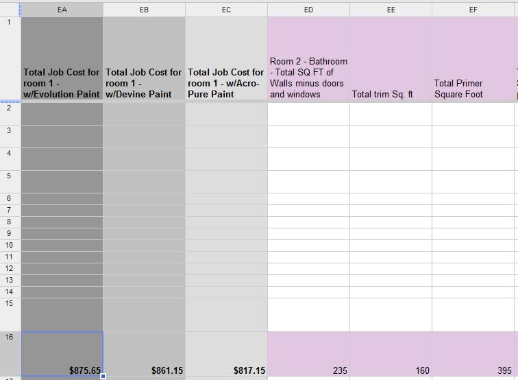
Part of Sheet1

Part of Sheet2

as exists now with formulas based on row 16 as a static row

Part of Sheet2

making row number used in the formulas as a variable

so for estimate for next row down 16 if changed to 17 will update results for row 17

yogi_Keep A Formula In Each New Record Row When Form Passes A New Record

Yogi Anand, D.Eng, P.E.                                         Google Spreadsheet                            www.energyefficientbuild.com

Delphi1 said:

When a form transfers data to its spreadsheet, it adds a new row but does not use the formula that I put in the previous record row.

I tried to fix this by copying the formula (vlookup) down 10 blank rows, but the next new record transferred from the form at row 11, below the blank rows with my formula in them.

How can I get the vlookup formula to stay in each new record?

My purpose;

Customer selects a Program Name from a drop down in the form.  The spreadsheet should then populate several cells, in the same record row, with part numbers and other lookup information using the vlookup formula.  But as each new record transfers into the spreadsheet, I have to manually copy/paste the formula into blank cells of the new record.

Any suggestions would be appreciated.

----------------------------------------------

Following is an image of the spreadsheet

Sheet1

I have created arrayformulas wherever you had computatiuons.I have created range name cross_reference as Sheet2!A4:E13 to take it out of the ResponseTable Sheet.

I have created range name cross_reference as Sheet1!E2:E80

Sheet2

formula in cell D2 is:

=ArrayFormula(transpose(split(concatenate(if(Alpha_PN=transpose(index(cross_reference,0,1)),transpose(index(cross_reference,0,2)),"")&char(9)),char(9))))

formula in cell F2 is:

=ArrayFormula(transpose(split(concatenate(if(Alpha_PN=transpose(index(cross_reference,0,1)),transpose(index(cross_reference,0,3)),"")&char(9)),char(9))))

formula in cell G2 is:

=ArrayFormula(transpose(split(concatenate(if(Alpha_PN=transpose(index(cross_reference,0,1)),transpose(index(cross_reference,0,4)),"")&char(9)),char(9))))

formula in cell O2 is:

=ArrayFormula(transpose(split(concatenate(if(Alpha_PN=transpose(index(cross_reference,0,1)),transpose(index(cross_reference,0,5)),"")&char(9)),char(9))))

yogi_Compare TWO Columns To TWO Other Columns And Find Unique Values

Yogi Anand, D.Eng, P.E.                                         Google Spreadsheet                            www.energyefficientbuild.com

ohthatdeb said:
There are two lists.
List 1 = Column A + Column B
List 2 = Column D + Column E
And the result I want (shown in Columns G & H) is a list of all items in List 2 that DO NOT appear in List 1.
For example, List 1 has two types of orange:
Orange, Cara Cara
Orange, Blood
List 2 also has two types of orange:
Orange, Cara Cara
Orange, Navel
I need to know which types from List 2 I should add to List 1 to make a complete list.
Both lists contain Cara Cara, but List 2 also contains Orange, Navel which does NOT appear in List 1, so I want that one in my result.
Hope that makes sense -- thanks for looking at it!
---------------------------------------------------------------------

yogi_Create Different Operations Based On A Set Of Criteria

Yogi Anand, D.Eng, P.E.                                         Google Spreadsheet                            www.energyefficientbuild.com

gffcnnn said:

Create different operations based on a set of criteria?
Hopefully I can explain this; I have tried using IF, IFERROR and AND statements, but I'm getting nowhere.
I would like three cells:
One is an "input" cell which will contain a decimal between 0 and 1
The other two are the "big" and "small" product cells. (The "big" cell will be added to by a different formula also.)
The criteria I need are these:
If the input is between 0.0 and 0.14, do nothing
If the input is between 0.15 and 0.42, add 1 to the "small" cell
If the input is between 0.43 and 0.64, add 2 to the "small" cell
If the input is between 0.65 and 0.85, add 1 to the "big" cell and subtract 1 from the "small" cell
If the input is between 0.86 and 0.99, add 1 to the "big" cell
I imagine this is a bunch of nested statements?
---------------------------------------------------------------------------------

yogi_If A Equals Y then C Equals B Else C Equals C

Yogi Anand, D.Eng, P.E.                                         Google Spreadsheet                            www.energyefficientbuild.com
anonymous user said:
I've looked around a lot but having no luck finding a straight forward answer. I know Google Docs doesn't allow iterative circular references like Excel and OpenOffice Calc do (GRR) but I need to import a sheet that does just that.
The data is Currently like this:
A B C
Y D =IF(A1=Y;B1;C1)
The formula copies down the entire sheet. Basically the idea is to only update collumn C if collumn A is a certain value, otherwise leave the currently displayed data in Collumn C alone. However, in Google Docs I can't use that formula since it doesn't allow iteration.
I'm trying to find a way to do the same thing within the bounds of Google Docs but having no luck. Any help would be appreciated. Using additional hidden cells would be fine but I'm not sure how to do that either, everything I have come up with thus far winds up with a circular reference.
Any help would be appreciated.
----------------------------------------------------------------------------------
Let us say the following image depicts the original data in columns A, B, and C

In the following solution I have used an additional column D ... column C can be optionally hidden.

yogi_Add SalesTax Only For Specified State

Yogi Anand, D.Eng, P.E.                                         Google Spreadsheet                            www.energyefficientbuild.com
unibox said:
I have a form that creates a customer database, i think thats what it would be called. It's for a small carpet cleaning business. I enter the jobs sorted by date booked. I need to add .05% tax to WI and not IL.
I have columns for- street address, State, Sub total, WI Tax, Total.
I'd like to have it know when State is WI then Sub total*.05 = WI tax then take WI tax and add to Sub total= total
else Sate= IL then sub total = total
Geezz that is a rambling mess. I hope I was clear enough..
---------------------------------------------------------------------------------
In the following solution I have generalized the State of interest to be housed in cell T2 and I have used a single array formula to populate needed entries in columns P and Q according to unibox's specification

yogi_Make A Survey And See The Overall Score For Each Respondent

Yogi Anand, D.Eng, P.E.                                   Google Spreadsheet                      www.energyefficientbuild.com

Taco Bos said: 

I'm working on a self test containing ten multiple choice questions. Each answer gives a certain score, and I'd like to automatically calculate an overall score for each respondent.
I'm thinking of the following solution:
- Replace all answers in the spreadsheet with scores
- Add up the scores for each contestant
The thing is: I don't know how I can replace certain answers for scores for each question (different questions have different scales).
I hope you can help, or maybe you see a different solution.
I use the form feature indeed, and I'm working on a translated (into Dutch) version of the Edinburgh Depression Scale: 

http://www.shiregps.org.au/documents/MH_Edinburgh_PND%20Scale.pdf

As you can see in the PDF, each answer has a score and sometimes the first answer gives the lowest score, and with other questions the first answer gives the highest score. In Google Docs, I'd like to translate the given answers into the applicable scores without a lot of manual work for each respondent. How can I use formulas to give the right scores to the different answers? 

------------------------------------------------------

In the following illustration I have used three questions ... each question is a multiple choice question with 4 options. Questions 1 and 2 have a score of 0,1,2, and 3 for options 1 through 4 respectively and question 3 has score of 3,2,1, and 0 for each of the options respectively. I created the Form originally for the fields shown with Gray headers and then later on I added additional columns with brown colored background for formulas for scores by question and then a column with yellow colored header for Total Scores for each respondent.

------------------------------------------------------------------------------
here is the Form that was created for this illustration

-----------------------------------------------------------------------------
and in the following I present the Summary of responses

yogi_Sum Values In A Column For A Group Matching Numbers In Another Column

Google Spreadsheet

nomedeusuario said:
I have a situation where I want to have a sumif, where my "condition" is a group and not one variable.
For instance:
Group A:
1
2
3
Activities
A1: 1 B1: 10
A2: 4 B2: 5
A3: 3 B3: 5
A4: 2 B4: 4
A5:5 B5: 5
A6: 1 B6: 1
A7:6 B7: 2
Target:
To build a Sum Group A function that will return in this case 10 + 5 + 4 + 1
Is that possible to achieve that with the Query function ? how ?
--------------------------------------------------------------------------------
In the following I have solutions using the SUMIF function, the FILTER function, and the QUERY function

yogi_Create An Arrayformula That Displays Only Unique Submitters

Yogi Anand, D.Eng, P.E.                                         Google Spreadsheet                            www.energyefficientbuild.com

yachdhoo said:
Column B Lists names of user submissions, which continue to grow.
Unfortunately, these do not represent unique users, as some have the same name.
Furthermore, each user submits more than once, and sometimes under a different name each time! (nick name, initials, etc).
Column C is a URL for each user, ending in that user's unique 9-12 digit alphanumeric, as in:
http://www.xxx~~~php?id=123xyz789
(The URL might be different for each user each time, but not the Unique identifier at the end, after the "=")
So, this 9-12 digit alphanumeric is the only way to correctly identify a unique submitter.
Therefore, on another sheet, I'd like to have one arrayformula that results in one row for each unique user (based on the 9-12 digit alphanumeric at the end of the URL they submit) with just two columns of data, auto-populating with additional submissions:
Column A with their names hyperlinked to a specific alternate URL ending in their alphanumeric (hyperlink("http://www.newphp?id=123xyz789","Name Submitted")
Column B with just their unique 9-12 digit alphanumeric, which is at the end of the URL they submit, after a "=").
...and where B has two entries for A, just return the most recent A (if different by way of initials, nickname, fullname, etc...)
Is this possible?
-------------------------------------------------------------------

yogi_Count Objects In An Array Tthat Match Another Array In Different Size

Yogi Anand, D.Eng, P.E.                                 Google Spreadsheet                    www.energyefficientbuild.com

Santiago said:
Count objects in an array that match another array in different size.
I'm working on a dashboard and I have 2 arrays. One with unique values and another one with many values that match the first array. I want to know how many values in the second array match the values in the first array. I know how to do this on VBA, but I'm not allow to use it.
Here is the example:
Array1={a,b,c}
Array2={a,a,a,r,t,y,c,b,b}
here, the result of what I want would be 6 (3 a, 2 b and 1 c)
I appreciate any help.
reference:
http://www.linkedin.com/groupAnswers?viewQuestionAndAnswers=&discussionID=53050779&gid=3124035&commentID=38525014&goback=%2Egde_3124035_member_52807150&trk=NUS_DIG_DISC_Q-ucg_mr#commentID_38525014
------------------------------------------
Following is a solution is Sheet1 using Google Docs Spreadsheet

yogi_ Change Date Text To Date Format

Yogi Anand, D.Eng, P.E.                                         Google Spreadsheet                            www.energyefficientbuild.com

PRASAD TR said:
Change Date Text to date format
How can we convert date format
From this
04-12-2011 04:37:00
04-12-2011 12:57:00
04-12-2011 11:37:00
To this
04-Dec-11
04-Dec-11
04-Dec-11
With out doing following things.
#should not copy past in notepad and copy back to excel.
#Should not remove Time.
it's not coming even if do Right click "Format Cells".
Kindly suggest . if past this data in sheet1 it should be automatically change to date format.
reference:
http://www.linkedin.com/groupItem?view=&srchtype=discussedNews&gid=3124035&item=52807150&type=member&trk=eml-anet_dig-b_pd-ttl-cn
---------------------------------------------------------------------------------