yogi_Pull In 'Single Case' Child Stats By Querying 'Raw Data' By Parent First Name

                                         Google Spreadsheet   Post  #1649
Yogi Anand, D.Eng, P.E.      ANAND Enterprises LLC -- Rochester Hills MI     www.energyefficientbuild.com.   May-26-2014
post by Bruce Gale: (https://productforums.google.com/forum/#!mydiscussions/docs/2nQ9bYqQlRs)
Dynamically changing row numbers in a formula

I have created a short (2 min) video that indicates what I am trying accomplish.  Credits to this forum, because my original request was going to be how to use the "OR" function in an array, but I resolved that.  On to business....

I wish to point to a single row as part of a formula.  Click below to view the video (hopefully it has processed by the time this is viewed, otherwise requires a download to view):

http://goo.gl/1cjZvE

Thanks for any assistance you can provide.

Bruce

---

Okay thanks, I have removed the original data.  This is what I am trying to accomplish.

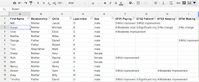
Here is the sample spreadsheet

http://goo.gl/FKn3EN

I have Raw Data containing multiple children who have been rated, e.g., Susan" in row 3 below

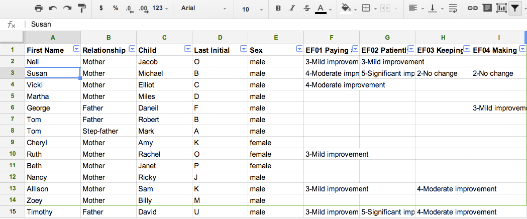
I want to be able to extract data from a single case as below, as appears in the spreadsheet Single Case

=TRANSPOSE('Raw Data'!A15:I15)

but switch from one row to another without having to change all of the numbers (e.g., row 15).  

Somehow I need a variable to point to the correct row to make the data dynamically change from one case to another.  Then the filter in subsequent spreadsheets will all reflect that single rater/case.  

=FILTER('Single Case'!A2:B11,('Single Case'!B2:B11 = "5-Significant Improvement")+('Single Case'!B2:B11 = "4-Moderate Improvement"))

E.g., switch from row 3 in Raw Data (Susan) to row 5 (Martha) to get those results.

Please let me know if I need to clarify further.  And thanks for any help you can provide.

Bruce

--------------------------------------------------------------------------------------------------------------------------------------------------

yogi_Pull List Of Unique Items In Columns D to F With Their Corresponding Count From Most To Least In Alphabetical Order

                                         Google Spreadsheet   Post  #1648 
                                     Updated Aug-01-2016 -- Added Sheet3

Yogi Anand, D.Eng, P.E.      ANAND Enterprises LLC -- Rochester Hills MI     www.energyefficientbuild.com.   May-25-2014
post by romgl: (https://productforums.google.com/forum/#!category-topic/docs/spreadsheets/O9TCwKC5fPs)
How to list and count unique cells in multiple columns?

Hi,

I'm wondering how you list and count the number of unique cells when they're in multiple columns and in a different tab. What formula would you use?

(I have data listed in columns D-F in one tab, and there are some repeats in different columns. I want to see which ones are repeated the most and how many times)

Thanks!

---

'm sorry, I don't want to make my spreadsheet public.

I did find a formula through a Google search which works for all the data in one column, but I don't know how to modify it for three columns. The formula I found was this:

=query(query('Bonuses'!$D$1:$D;"select D, upper(D) where (D is not null and D<>'')";0);"select Col1, count(Col2) group by Col1 order by count(Col2) desc label count(Col2) 'count'";1)

Do you know how to change this so that it works for columns D-F, and not just D?

--------------------------------------------------------------------------------------------------------------------------------------------------

yogi_Apply Conditional Formatting To Highlight Second or Higher Instance Of A Name (duplicates) In A Column

                                         Google Spreadsheet   Post  #1647
Yogi Anand, D.Eng, P.E.      ANAND Enterprises LLC -- Rochester Hills MI     www.energyefficientbuild.com.   May-24-2014
post by Cinthis Gordillo: (https://productforums.google.com/forum/#!category-topic/docs/spreadsheets/0KcYllc3UaU)
I need to find duplicates in the same column
I need to know how to find duplicates in the same column with manually delete option. 

Please help

----------------------------------------------------------------------------------------------------------------------------------------------------

yogi_Conditional Formatting For Tentative Launch Date When It Precedes A Specified Reference (Today) Date

                                         Google Spreadsheet   Post  #1646
Yogi Anand, D.Eng, P.E.      ANAND Enterprises LLC -- Rochester Hills MI     www.energyefficientbuild.com.   May-23-2014
post by BryanP -- question by sricha: (https://productforums.google.com/forum/#!mydiscussions/docs/OsjqOTXZQl4)
New Conditional Formatting option - Custom formula is
Hello,

Wanted to check if today() function can be used within custom formula of conditional formatting? I am trying this query which otherwise works fine-

=if(F3<TEXT(left(today(),1)/3, "0.0")))

Appreciate any help.

--

thanks

Richa

---

Thanks for looking into it Yogi !

I am trying to highlight a cell based on its current status.

Details-

One cell contains product's tentative launch date. Another cell contains actual launch date.

I need to highlight 1st cell in red when today's date is > 'tentative launch date' and 'actual launch date' is null

---------------------------------------------------------------------------------------------------------------------------------------------

yogi_Convert Math Formula For Measuring Distance Between Two Points To Spreadsheet Formula

                                         Google Spreadsheet   Post  #1645
Yogi Anand, D.Eng, P.E.      ANAND Enterprises LLC -- Rochester Hills MI     www.energyefficientbuild.com.   May-20-2014
post by bqs onaquest2: (https://productforums.google.com/forum/#!category-topic/docs/spreadsheets/hve5sNpf_ic)
help converting formula to measure distance between 2 points to spreadsheet

Okay I just want  to convert the Pythagorean theorem  in to a formula google spreadsheets can read.  I'm trying to measure  the distance between two points on a graph.  I have provided a link that explains formula simply for those not familiar or have forgotten. I also included a image of the actual  formula... I just need to know how to make it pull from cells and spit out answer in a different cell.

Link: http://www.mathsisfun.com/algebra/distance-2-points.html

------------------------------------------------------------------------------------------------------------------------------------------------------------------

yogi_ Count Number Of Items By Type From Multiple Items In Each Type

                                         Google Spreadsheet   Post  #1644
Yogi Anand, D.Eng, P.E.      ANAND Enterprises LLC -- Rochester Hills MI     www.energyefficientbuild.com.   May-20-2014
post by Samford: (https://productforums.google.com/forum/#!mydiscussions/docs/6k2s4kRVz4g)
Counting multiple criteria - formula works in old version of sheets but not the new!

Can anyone explain why this formula:

=sum(countif(C8:C12,{"DCP","CO2","WC","F","FM"}))

... works perfectly in the old version of Sheets and counts all the criteria listed, but when applied in the new Sheets - it doesn't work properly.

Here's how it looks in the new version of Sheets:

=sum(countif(C12:C25,{"DCP","CO2","WC","F","FM"})) This formula in the new Sheets only returns the number of items listed as "DCP" which is only the first criteria listed.

What has changed???

Any help is most appreciated!

---

Hi Yogi

thank you so very much for looking at this problem for me.  I tried your suggestion and it returned a value of "0" - which is not correct.

Here is a link to the spreadsheet, if that helps:

https://docs.google.com/spreadsheets/d/1Gpmry5OuwM-oHGS4Mor_U4s3M-MZ7EkIz9_a3V-jeJI/edit?usp=sharing

Thanking you in advance..

--------------------------------------------------------------------------------------------------------------------------------------------------------

yogi_Apply Conditional Formatting To Specified Range (A2 to D5) Based On Values In Column C

                                         Google Spreadsheet   Post  #1643
Yogi Anand, D.Eng, P.E.      ANAND Enterprises LLC -- Rochester Hills MI     www.energyefficientbuild.com.   May-20-2014
post by vincentvc -- question by zander Bingle: (https://productforums.google.com/forum/#!mydiscussions/docs/t6xPcOkjNbQ)
Conditional formatting cell to entire line

Hi Yogi

You'll see I've got two example tables, using the indirect formula, it works perfectly (first table). When using a straight forward relative reference, it doesn't work at all :/ It's basically assuming that you you want to validate the formatting for the whole table based on that one cell only, yet only formats the first cell in the specified range.

I don't know if Google is planning on changing the manor in which Conditional Formatting will react when formatting a whole table based on a single column. I know for a fact that there are very little people aware of the indirect function, even in Excel.

Example document:

https://docs.google.com/spreadsheets/d/1mELOR9bxYyuBjpjh0n8zNCUAFRyQ4XqIfrC7pdzB3x0/edit?usp=sharing

Please let me know should you require any additional information.

I've only recently started using Google docs, loving it and tinkering for personal use only. So it's not a train smash ;)

Kind Regards

Zander Bingle

----------------------------------------------------------------------------------------------------------------------------------------------------------

I think the question by implications is ... must one use INDIRECT function in such a case as Zander has used --

my following illustration shows that one does not necessarily need to use the INDIRECT function