Sunday, March 9, 2014

yogi_Compute Sum In Column C Based On startDate And endDate entries in Column B

                                         Google Spreadsheet   Post  #1555
Yogi Anand, D.Eng, P.E.      ANAND Enterprises LLC -- Rochester Hills MI     www.energyefficientbuild.com.   Mar-09-2014
post by Yarra Liebermann-Cliff   (https://productforums.google.com/forum/#!category-topic/docs/spreadsheets/pjgWGpJnars)
Summing a range based on a range of dates
Hey guys,

I'm a freelance writer and I'm trying to be responsible and check my salary. To do that I've tried using Google Sheets formulas with no apparent success, so I'm turning to you.

Basically, I have column A (range name=name) with the subject of the article, column B (range name=date) with the date it was published on, and column C (range name=money) with the amount of money I received for that article.
Now, I get paid in April for every article that was published between 20/01/2014-20/02/2014. 
I want to find a formula that will calculate the sum within the range money based on the right range in date. The thing is I couldn't find the right way to do so and I really don't want to manually change the regular sum() formula when I add an item to the data...


Disclaimer: the document is in Hebrew but ranges are in English and also I'm using columns here so it should be no problem.
-------------------------------------------------------------------------------------------------------------------------------------------------------


yogi_Query And Pull From Google Form Data Select Columns For Today Entries Meeting Additional Criteria

                                         Google Spreadsheet   Post  #1555
Yogi Anand, D.Eng, P.E.      ANAND Enterprises LLC -- Rochester Hills MI     www.energyefficientbuild.com.   Mar-09-2014
post by Andy Chaplin (https://productforums.google.com/forum/#!category-topic/docs/spreadsheets/1eI9BjrYQDk)
Making a query based on on today's results
ve been using the query function for a while now and with the help files and the forums have managed to solve most problems, but this one is driving me crazy!

I need to do a query which just shows today's entries from a Form.  The timestamp is in Col A.  I've tried various combinations of date, dateDiff, toDate, now(), and today() but just get parse errors.  My latest attempt was this:

=QUERY(Consolidation!A2:W1000, "select B, P, Q, R, S where dateDiff(now(), A) = 0 and T = 'Krankmeldung'")

The strange thing is that when I used "> 1" in the above formula, it showed all the old results, but "= 0" throws an error.

Can anyone tell me what I am doing wrong?

Thanks for any help!
---------------------------------------------------------------------------

Saturday, March 8, 2014

yogi_Multi-Conditional Sum Of Amounts Of Various Categories By Months Of The Specified Year

                                         Google Spreadsheet   Post  #1554
Yogi Anand, D.Eng, P.E.      ANAND Enterprises LLC -- Rochester Hills MI     www.energyefficientbuild.com.   Mar-08-2014
post by Jeffrois  (https://productforums.google.com/forum/#!mydiscussions/docs/KBH3YRKe6oM)
Nested SUMIF (or possible other function) with month/date range
I'm trying to do a nested SUMIF, but to no avail. This is what I'm trying to accomplish

I'm trying to add the amount (column F) based on category (G) AND month (B). The end goal is going to have a separate cell for every month/category combination. For example, for the month of September, I will have a separate cell (and a separate code) for Miscellaneous, Inventory, etc. For the month of October I'll have a separate cell for the same. So, the SUMIF (or other function) would need to include a range of cells (currently B3:B33 for the date, G3:G33 for the category, and F3:F33 for the amount that will be totaled).


I can get a month function to work -- =IF(MONTH(B5)=9,"yes","no") and a sumif function to work, but not the combination of the two.

Any thoughts or ideas? Please let me know if you need any more info.

Thanks for your help!

---
Hi Yogi,

Thanks for being willing to take a look at it! It looks like the image that I posted didn't get published correctly anyway.


When looking at that document, the formula would go in the tab, "Cash Flow", in cell D9 for Inventory, D10 for Rent, D11 for Wages, etc. Once the D column is complete, I would drag the formula to the right for the remaining months and update as needed. The formula would relate to the "Investments" tab. Again, needing to total sums in the "Total column, depending on each category (Rent, Wages, Marketing, Miscellaneous, etc), as well as the month.

By the way, I've checked out your blog in the past when I've had questions, and I appreciate your posts! Thank you!

Please let me know if you need any more info.

Best,

Jeff
----------------------------------------------------------------------------------------------

Thursday, March 6, 2014

yogi_Apply Conditional Formatting to Highlight Lowest Price of Part Row By Row

                                         Google Spreadsheet   Post  #1553
Yogi Anand, D.Eng, P.E.      ANAND Enterprises LLC -- Rochester Hills MI     www.energyefficientbuild.com.   Mar-06-2014
post by rickprendergast  (https://productforums.google.com/forum/#!mydiscussions/docs/d8eU-paF08k)
Conditional Formatting - Comparing one value to multiple values
Hi,
I am using the new Google Sheets and I am trying to compare multiple values and change the background of the lowest value to green.
Here is a sample of what I am doing.  I would like to make the cell with the lowest price for each part turn green.
Thanks for your help.

Rick

PART NUMBERICCNEWEGGPROVANTAGE
9260-4i367.20294.99301.78
9271-4i386.64383.99381.29
9260-8i468.72479.00477.38
9271-8i528.12511.90530.92
LSIIBBU07 (9260)158.22156.99171.43
LSICVM01 (9271)208.44176.99188.13

-------------------------------------------------------------------------------------------------------------------

Wednesday, March 5, 2014

yogi_Pick Column By Column The Name With Most Occurrences In The Column

                                         Google Spreadsheet   Post  #1552
Yogi Anand, D.Eng, P.E.      ANAND Enterprises LLC -- Rochester Hills MI     www.energyefficientbuild.com.   Mar-05-2014
post by PKnowles13  (https://productforums.google.com/forum/#!category-topic/docs/spreadsheets/rFZ9zm0Tubw)
Tally most frequent response

Monday, March 3, 2014

yogi_Apply Conditional Formatting To Cells Of Column A For Blue And Bluish -- sort of like using wildcard with Blu

                                         Google Spreadsheet   Post  #1551
Yogi Anand, D.Eng, P.E.      ANAND Enterprises LLC -- Rochester Hills MI  www.energyefficientbuild.com  Mar-03-2014

Updated Sep-17-2016

post by rossmcm (https://productforums.google.com/forum/#!category-topic/docs/spreadsheets/VX_C5cek2Bk)
Syntax for conditional formatting expressions in the new sheets
I'm using the new sheets and want to add conditional formatting with a custom formula to a cell.  Can anyone point me at reference docs for the syntax of these expressions?


Feel free to have a play.
 TIA 
-----------------------------------------------------------------------------------------------------------------------

Sunday, March 2, 2014

yogi_Display Value From A Range Withourt Spreadsheet Title Or Sheet Name Using Google Old Sheet

                                         Google Spreadsheet   Post  #1550
Yogi Anand, D.Eng, P.E.      ANAND Enterprises LLC -- Rochester Hills MI 
post by Abby Rudakov (https://productforums.google.com/forum/#!category-topic/docs/spreadsheets/-4p1vG4tGbQ)
Help displaying value from Google Spreadsheet online
Hi,

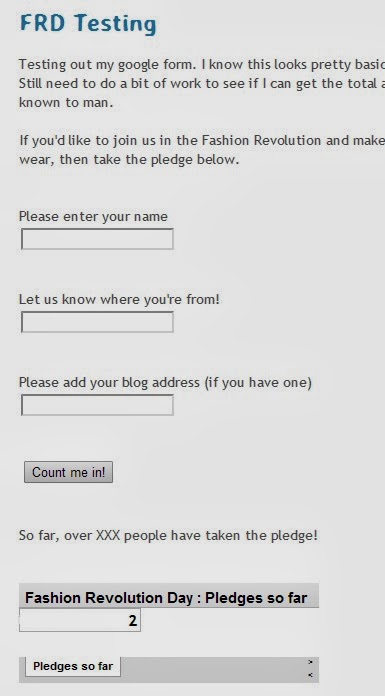
I've got a Google Form setup which takes people's details. In the Google Spreadsheet, I am calculating the total number of entries (via a count of the timestamps) and I would like to be able to display the total number online, specifically on a Blogger blog post. I have been able to figure out how to show the tab from my spreadsheet with the number, but it looks super ugly and I'm only really after the number not the headers and page tabs too. Any suggestions? TIA

---------------------------------------------------------------------------------------------------
in the following I present the iframe code to publish value from a range without spreadsheet title or sheet name using Google Old Sheets. You will have to adjust the width of the range to be published, the font color and background color to suit your need and/or preference.

to publish cell B2 with spreadsheet name and sheet name the iframe code is
<iframe width='500' height='300' frameborder='0' src='https://docs.google.com/spreadsheet/pub?key=0AkHBcyclu11AdGJZM2tRUjdlVFJVaXFJemhUUzZxcUE&single=true&gid=3&range=B1&output=html&widget=false'></iframe>
formula in cell B1
="so far over "&count('Form Responses 1'!A:A)&" people have taken the pledge"


I  am also posting here all the sheets from Abby's spreadsheet