Saturday, December 21, 2013


Sunday, December 15, 2013
yogi_Compute Jerry Seinfeld Chain From A Set Of Current Streaks
Google Spreadsheet Post #1440
Yogi Anand, D.Eng, P.E. ANAND Enterprises LLC -- Rochester Hills MI www.energyefficientbuild.com. Dec-15, 2013
question by Josiah Sprague (http://productforums.google.com/forum/?zx=2prcm5ppprxr#!mydiscussions/docs/wBleMdlhsWM)
Formula for calculating a running average of streak length
I'm using Jerry Seinfeld's chain method to track habits that I want to change. I want to track my chains in a Spreadsheet and have a running average of my chain length. I want to be able to say something like, "On average, over the last six months, the length of my 'winning streaks' has gone up/down".
Yogi Anand, D.Eng, P.E. ANAND Enterprises LLC -- Rochester Hills MI www.energyefficientbuild.com. Dec-15, 2013
question by Josiah Sprague (http://productforums.google.com/forum/?zx=2prcm5ppprxr#!mydiscussions/docs/wBleMdlhsWM)
Formula for calculating a running average of streak length
I'm using Jerry Seinfeld's chain method to track habits that I want to change. I want to track my chains in a Spreadsheet and have a running average of my chain length. I want to be able to say something like, "On average, over the last six months, the length of my 'winning streaks' has gone up/down".
I have a vague idea of how to set this up, but I am not quite there. I've got one column for date, another column for the current streak length on each day, and I'm trying to come up with a third column that will generate a running average of my streak lengths over a certain time period (say 6 months). Eventually I would like to graph this information too, so that I can see how my average streak length is changing on a daily basis. I'm at a loss for which formula to use, or perhaps I need to tweak my model a little bit to get the information I am looking for.
Any help would be greatly appreciated!
-----------------------------------------------------------------------------------------------------------------------------
yogi_Multi_Conditional Count of Pokemons Of Type1 or Type2 And Stage Basic or Baby
Google Spreadsheet Post #1439
Yogi Anand, D.Eng, P.E. ANAND Enterprises LLC -- Rochester Hills MI www.energyefficientbuild.com. Dec-15, 2013
question by Paul Toro (http://productforums.google.com/forum/?zx=2prcm5ppprxr#!mydiscussions/docs/0wFkFZ3N-N4)
Counting up unique terms if they meet requirements. replacing countifs
Yogi Anand, D.Eng, P.E. ANAND Enterprises LLC -- Rochester Hills MI www.energyefficientbuild.com. Dec-15, 2013
question by Paul Toro (http://productforums.google.com/forum/?zx=2prcm5ppprxr#!mydiscussions/docs/0wFkFZ3N-N4)
Counting up unique terms if they meet requirements. replacing countifs
I'm making a data chart using some formula I found to add up unique data from two columns and return them to one, followed by a count of the number of times those unique items occur.
This is that formula i found and am using to get data from two columns, it seems to work fine.
=ArrayFormula(unique(transpose(split(concatenate( C3:C151&char(9),D3:D151&char( 9)),char(9)))))
This is the Count I'm using now.
=COUNTIF($C$3:$D$151;A166)
However, now I only want it to count up the unique term if it first checks the cell in a column next to it in the same row, and if that cell has one of the two correct unique terms out of the many possible.
This is what I attempted to do.
=COUNTA(FILTER(C3:D151;F3:
I want it only to count things from that same group, "c:3:d151" known also as two separate column ranges I called Type1 and Type2 (but i have yet to use them this way because I'm not very good), if the corresponding cell in the F column (i called this range 'Stage'), contains the word red or blue. A166 is where the term it should be counting is listed. As you can see, mine doesn't work.
How can I add this condition to the count if? I am using google spreadsheet right now but I'd like it to work on Excel too. I would really appreciate the help, it's information I would use for a long time. Any information on why mine doesn't work and yours does would be even better. Thankyou.
--------------------------------------------------------------------------------------------------------yogi_Compute Sum Numbers In Labels (Row 2) For Corresponding X Marked Items In Row 3
Google Spreadsheet Post #1438
Yogi Anand, D.Eng, P.E. ANAND Enterprises LLC -- Rochester Hills MI www.energyefficientbuild.com. Dec-14, 2013
question by chris4mac (http://productforums.google.com/forum/?zx=8wfymr6zg7vv#!category-topic/docs/spreadsheets/OWn-N1ZRUUg)
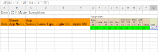
I want to assign numeric values to text entries and sum a string of cells
Yogi Anand, D.Eng, P.E. ANAND Enterprises LLC -- Rochester Hills MI www.energyefficientbuild.com. Dec-14, 2013
question by chris4mac (http://productforums.google.com/forum/?zx=8wfymr6zg7vv#!category-topic/docs/spreadsheets/OWn-N1ZRUUg)
I want to assign numeric values to text entries and sum a string of cells

What I want to do is simple. I want my clients to be able to mark tasks with an "x". Each task has a monetary value associated with it. Since the monetary value is listed at the top - all I need them to see is the SUM of the costs. However, whether I try to substitute x for the appropriate value, the process quickly erodes. I have also tried IF, or "Replace", but I cannot find a way to accomplish this task. HELP PLEASE!
----------------------------------------------------------------------------------------------------------------yogi_Count Incidents By CrossTabbing Antecedent and Behavior From Patterns Noted In Form Responses Sheet
Google Spreadsheet Post #1437
Yogi Anand, D.Eng, P.E. ANAND Enterprises LLC -- Rochester Hills MI www.energyefficientbuild.com. Dec-14, 2013
question by Benjamin Yamato (http://productforums.google.com/forum/?zx=8wfymr6zg7vv#!category-topic/docs/spreadsheets/WYjVaSMgx5g)
Counting based on two criteria in a table.
Yogi Anand, D.Eng, P.E. ANAND Enterprises LLC -- Rochester Hills MI www.energyefficientbuild.com. Dec-14, 2013
question by Benjamin Yamato (http://productforums.google.com/forum/?zx=8wfymr6zg7vv#!category-topic/docs/spreadsheets/WYjVaSMgx5g)
Counting based on two criteria in a table.
I'm looking for a way to create a table of data based on two criteria generated from a google form. I've attached the screenshot of the data I'm trying to use. The user selects items from two checkbox lists, so there can be multiple entries in a single cell. On a second worksheet (also attached), I'm trying to reference the data from the "Form Response" sheet to count incidents based on two criteria, which you can see in column/row headings.
I'm looking for the formula to put in the cells on the second worksheet. Based on googling/research, I've been trying to make this formula work:
=ARRAYFORMULA(SUM(('Form Responses'!$L:$L=$A2)*('Form Responses'!$U:$U=B$1)))
But it's just giving me a return value of "1", regardless of the data.
Thanks for any/all help!
Attachments (2)
Saturday, December 14, 2013
yogi_From Names And Weeks In Sheet1 Make A CrossTab By Name And Week In yogi_Sheet3 Showing completed not completed
Google Spreadsheet Post #1436
Yogi Anand, D.Eng, P.E. ANAND Enterprises LLC -- Rochester Hills MI www.energyefficientbuild.com. Dec-14, 2013
question by Johnson Controls (http://productforums.google.com/forum/?zx=iqfbvnd0jbz1#!category-topic/docs/spreadsheets/VvFMaUYoq6E)
IF Function for certain value then adjacent cell value
Yogi Anand, D.Eng, P.E. ANAND Enterprises LLC -- Rochester Hills MI www.energyefficientbuild.com. Dec-14, 2013
question by Johnson Controls (http://productforums.google.com/forum/?zx=iqfbvnd0jbz1#!category-topic/docs/spreadsheets/VvFMaUYoq6E)
IF Function for certain value then adjacent cell value
I want to look up in sheet1 columnA for a name(mike smith) then check cell beside his name for (week1) and if it is there then mark sheet3 cell(any cell as of now) completed, what I am trying to accomplish is that there are 52 weeks in the year and I have several people performing audits everyweek and want to keep track of auditers and which weeks they have completed (example below)
mike smith
Column A Column B
week1 completed
week2 completed
week3 not completed
---------------------------------------------------------------------------------------------
Wednesday, December 4, 2013
yogi_Merge Several Sheets Of A Spreadsheet Into yogi_COMPOSITE All Rows Where Textual Column I Of Merged Sheets Is Not Blank
Google Spreadsheet Post #1435
Yogi Anand, D.Eng, P.E. ANAND Enterprises LLC -- Rochester Hills MI www.energyefficientbuild.com. Nov 24, 2013
question by BTGov (http://productforums.google.com/forum/?zx=1kdqdmp9bh1u#!mydiscussions/docs/hRjM2vxYXoY)
How to display all values in a column across multiple sheets
I have a google spreadsheet with several sheets that are all formatted identically. Each sheet has it owns name relative to different accounts that I am tracking. Each sheet has the same column headers, but I want to generate another sheet with a formula that returns all values in column j for all sheets in document while excluding the blank cells.
---
Here is the link
Yogi Anand, D.Eng, P.E. ANAND Enterprises LLC -- Rochester Hills MI www.energyefficientbuild.com. Nov 24, 2013
question by BTGov (http://productforums.google.com/forum/?zx=1kdqdmp9bh1u#!mydiscussions/docs/hRjM2vxYXoY)
How to display all values in a column across multiple sheets
I have a google spreadsheet with several sheets that are all formatted identically. Each sheet has it owns name relative to different accounts that I am tracking. Each sheet has the same column headers, but I want to generate another sheet with a formula that returns all values in column j for all sheets in document while excluding the blank cells.
---
Here is the link
https://docs.google.com/
I basically want to have a sheet that shows all data in columns (B through I) across all sheets from "First" to "Last" when there is a value in column I.
Let me know what you think.
--------------------------------------------------------------------------------------------
Subscribe to:
Posts (Atom)