yogi_Find Associated District From Given Set of Road/Locality and District Data

Google Spreadsheet   Post  #2481

Yogi Anand, D.Eng, P.E.      ANAND Enterprises LLC -- Rochester Hills MI     Jul-26-2018

question by: Steven Goovaerts
https://productforums.google.com/forum/?utm_medium=email&utm_source=ba_notification#!topic/docs/jI1bs1T3skI;context-place=forum/docs

Please Help - Return cell data based on range search

Hi!

I am very new to this and was hoping someone may be able to help?

I have been trying and failing to come up with a way to search a cell value across a large data set and return the column title of the located cell as the result.

I have tried everything from VLOOKUP/HLOOKUP to INDEX and MATCH, to ARRAYS, but I am completely lost.

I have attached a sheet with an example data set.  It includes a table of district groups and individual road references within those districts.

Essentially, I would like to be able to search by a road reference in a cell (e.g. "ElBrto2") and have the results return the district it is in (e.g. Springfield).  Something like ... SEARCH RANGE FOR ... "ElBrto2" AND RETURN RELEVANT COLUMN HEADER.

I am sure there is a simple way around this, so apologies for asking something so basic.

Any help would be greatly appreciated :)  Thanks!

SHARED SHEET HERE: 

https://docs.google.com/spreadsheets/d/1LCm2eBtz7l9bYHhgiOERT1bkHaCFZuBMysZi8MgVOhc/edit?usp=sharing 

yogi_Query B27:C Where C=Value As Specified And Sort By B and C In Desc Order

Google Spreadsheet   Post  #2480

Yogi Anand, D.Eng, P.E.      ANAND Enterprises LLC -- Rochester Hills MI     Jul-26-2018

question by: guyute
https://productforums.google.com/forum/?utm_medium=email&utm_source=ba_notification#!topic/docs/dA21oBp67f4;context-place=mydiscussions
How can I count totals of items multiple columns when the items overlap in each column?

I'm wondering if you could help. I'm trying to record procedures being done by multiple people.  Ultimately, I want to get the total amount of each unique procedure each person has done.  They will do different number of procedures each time (i.e. sometimes just one, sometimes 2, sometimes 5, etc.)  

Here's an example of what I have set up

	Procedure 1	Procedure 2	Procedure 3	Procedure 4	Procedure 5
Tom	a	a	b	c	d
Jerry	b	a	c	d	e
Mickey	e	b	c
Minnie	a

Each procedure could be either a, b, c, d or e.

Tom, Jerry, Mickey, and Minnie are the people performing the combinations of procedures.

I want to total automatically each specific procedure (a, b, c, d or e) regardless of which procedure column it falls in.  In other words, I don't care if there are 3 "a"s in procedure 1 column and 2 "a"s in column 3.  I just want a way to get to the total of 5 "a"s for Tom, Jerry, Mickey or Minnie.  

Is there a better way to record the data rather than by creating 5 procedure columns?  If not, then is there a way to get a count of unique procedures in all 5 columns?

This is somewhat difficult to explain, so I apologize if I'm not doing it well.  Thanks for any help!

yogi_Conditionally Format By Date Groups With A Blank Line Between Date Groups

Google Spreadsheet   Post  #2479

Yogi Anand, D.Eng, P.E.      ANAND Enterprises LLC -- Rochester Hills MI     Jul-25-2018

question by: guyute
https://productforums.google.com/forum/#!topic/docs/9bJSSRpGbvY;context-place=forum/docs
How do I automatically sort by 3 sequential columns and add a colored dividing line?

I would like to automatically sort by 3 fields sequentially so that I don't have to highlight everything, then click data>sort range each time.

1. How can I have it automatically sort by multiple columns? First by date (column B), then by location (column I), then by time (column c)?

2. Also, I would like to have a colored line (bottom of rows 31, 32 and 39) dividing the different dates. If a colored line isn't possible, then an empty row.

Here is the link to the spreadsheet:

https://docs.google.com/spreadsheets/d/1PTMx97jvepEfuOxxrRHRjISHhE1w4ndGNlehFBTsMv0/edit?usp=sharing

The sheet is called "example 2 for totals"

The tab is called "autosort".

The top part of the table shows the data unsorted.

The lower part of the table shows it sorted with the horizontal line dividers in it.

THANK YOU!!

yogi_Conditionally Format Alternate Group Of Date Sets From TimeStamps In Colum F

Google Spreadsheet   Post  #2478

Yogi Anand, D.Eng, P.E.      ANAND Enterprises LLC -- Rochester Hills MI     Jul-22-2018

question by: Silas 7467
https://productforums.google.com/forum/?utm_medium=email&utm_source=ba_notification#!topic/docs/8W0yTkvSmr0;context-place=forum/docs
Highlight rows corresponding to non-uniform alternating dates

Hello, I'm relatively new to google sheets, and slowly gathering information. I was not able to find any real answers to my query, so I thought I should ask. It doesn't seem like a complicated request, so hopefully the answer is out there and simple.

I'm trying to highlight in an alternating fashion all the rows of like dates. 

All the rows with the same date I want highlighted one way

All the rows of the following date I want highlighted another way, and so on... 

Ideally this could be done with conditional formatting, but I have no idea how to create a formula for this.

https://docs.google.com/spreadsheets/d/1qmJg0hM9mfa4U-4mUWOvRU5EdAu-18aMjR8KsWxETv4/edit?usp=sharing

yogi_Find Date Of Every Last Specified Weekday (Tuesday) Of The Month Following The Date In Specified Cell (S3)

Google Spreadsheet   Post  #2477

Yogi Anand, D.Eng, P.E.      ANAND Enterprises LLC -- Rochester Hills MI     Jul-20-2018

question by: Patrick Lathrop
https://productforums.google.com/forum/?utm_medium=email&utm_source=footer#!topic/docs/moqqtpK4UYE;context-place=forum/docs
Last (weekday) of following month formula for creating payment schedules?
So, with a little help from the help community i was able to put together an Nth day occurrence script that cleverly  determines the weekday associated with an original date (S3) and then counts the number of days in the current month to produce an accurate 1st 2nd 3rd or 4th (weekday) occurrence.

Unfortunately this clever bit of work, while accurate up to 2102 in my testing for 1st~4th occurrences gets broken by people who are assigned a last (weekday) of month schedule.

The current formula is as follows:

ARRAYFORMULA(S3+LOOKUP(COUNTIF(WEEKDAY(ROW(INDIRECT("M"&EOMONTH(S3,-1)+1&":M"&EOMONTH(S3,0)))),WEEKDAY(S3)),{4,5},{28,35}))
Is there a clever way to retrofit this formula to work with a LAST (weekday) payment schedule? Or an easier way to make a separate formula to detect the weekday and display the last weekday of the following month?

As example 7/31 (TUESDAY) and display 8/28/18 aka the last Tuesday of august 2018?

I'm including a copy of the spreadsheet i'm working on for reference, any and all help is greatly appreciated.

https://docs.google.com/spreadsheets/d/1MwKO0ZrRt9tw9yuFxyaVDI9PnvmicPj7Nq7PoWSjqhY/edit?usp=sharing

yogi_Extract Entity Values For Specified Item From Data In Another Sheet

Google Spreadsheet   Post  #2476

Yogi Anand, D.Eng, P.E.      ANAND Enterprises LLC -- Rochester Hills MI     Jul-16-2018

question by: Remember 13
https://productforums.google.com/forum/?utm_medium=email&utm_source=ba_notification#!topic/docs/dlq8Fc_kEEI;context-place=mydiscussions
Extract values from other sheets depending on another value + Transpose
Hi, 

I have this spreadsheet I'm sharing with 3 different tabs. There are formulas linking two of them ('Raw' and 'Measurements + Selling description') and I would like to extract data from tab 'Measurements + Selling description' to tab 'Description template' based on the item number I write on cell B1 of this last mentioned tab.

Basically I need to figure out the formula to be typed on 'Description template' cell F2 to get the value from 'Measurements + Selling description' cell H3 if I type 1 on 'Description template' cell B1. (I need it to extract the Description information for item 1 in that case). With that formula I would be able to apply the same formula for the other characteristics and use individual formulas for the Measurements which now have a "TRANSPOSE" simple formula.

What I'm doing right now is type it individually for each item every time I need it, but i'm sure it would be much faster if I can find out how to do it this way.

Thanks very much in advance for the help.

This is the spreadsheet:

https://docs.google.com/spreadsheets/d/1pKi0XcrrzmJNILS-LJyM696GG9-uiOuajJUOfQ4U3uI/edit?usp=sharing

yogi_Compute Average Waiting Time Hour By Hour From Check-In And Attended Times

Google Spreadsheet   Post  #2475

Yogi Anand, D.Eng, P.E.      ANAND Enterprises LLC -- Rochester Hills MI     Jul-15-2018

question by: Kyle Sylverne
https://productforums.google.com/forum/?utm_medium=email&utm_source=best_answer_notification_button#!topic/docs/OUD4eaDlgoM;context-place=forum/docs
Formula to filter timestamp when averaging
Hello,

I'm attempting to average wait times and want to filter the average based on the timestamp down to the hour. Below is a test spreadsheet of what I'm using. I'd like average column E (wait time duration) but filter the values based on column b's hours (so 6am, 7am, etc) I've attempted to try and play with the syntax and formulas and haven't been able to quite figure it out. 

Thanks

https://docs.google.com/spreadsheets/d/1wFVUcIK5-cxQFMyX-AbwkrB_AmAZOVfs05PnFprgGWQ/edit?usp=sharing

yogi_List Unique Values In Column A And Concatenate corresponding Values In Column B

Google Spreadsheet   Post  #2474

Yogi Anand, D.Eng, P.E.      ANAND Enterprises LLC -- Rochester Hills MI     Jul-14-2018

question by: Joshua Lingan
https://productforums.google.com/forum/?utm_medium=email&utm_source=ba_notification#!topic/docs/fHyHV4qmTCk;context-place=forum/docs
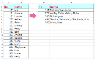
List Unique Values And Concatenate Corresponding Values??

I want to do something similar to this, but on Google Sheets. How would I go about doing it?

here is the link for a sample sheet: https://docs.google.com/spreadsheets/d/1yopKwn3vAJpgqbhLg8UFB2DmM4IjbP9YC8i2Qu6-g6w/edit?usp=sharing

I would use e-mail address column as the lookup value (unique value?) and Date Attended as the corresponding value..

So something like email | Date Attended (all values without adding duplicate values)

And if possible for the Date Attended values to be separated by a ";"

yogi_Multi-Criteria Count Problem 2

Google Spreadsheet   Post  #2473

Yogi Anand, D.Eng, P.E.      ANAND Enterprises LLC -- Rochester Hills MI     Jul-08-2018

question by: guyute
https://productforums.google.com/forum/?utm_medium=email&utm_source=best_answer_notification_button#!topic/docs/dA21oBp67f4;context-place=mydiscussions

How can I count totals of items multiple columns when the items overlap in each column?

I'm wondering if you could help. I'm trying to record procedures being done by multiple people.  Ultimately, I want to get the total amount of each unique procedure each person has done.  They will do different number of procedures each time (i.e. sometimes just one, sometimes 2, sometimes 5, etc.)  

Here's an example of what I have set up

	Procedure 1	Procedure 2	Procedure 3	Procedure 4	Procedure 5
Tom	a	a	b	c	d
Jerry	b	a	c	d	e
Mickey	e	b	c
Minnie	a

Each procedure could be either a, b, c, d or e.

Tom, Jerry, Mickey, and Minnie are the people performing the combinations of procedures.

I want to total automatically each specific procedure (a, b, c, d or e) regardless of which procedure column it falls in.  In other words, I don't care if there are 3 "a"s in procedure 1 column and 2 "a"s in column 3.  I just want a way to get to the total of 5 "a"s for Tom, Jerry, Mickey or Minnie.  

Is there a better way to record the data rather than by creating 5 procedure columns?  If not, then is there a way to get a count of unique procedures in all 5 columns?

This is somewhat difficult to explain, so I apologize if I'm not doing it well.  Thanks for any help!

yogi_From 1st of the Month and Year Compute Week Nos for The Month And Year

Google Spreadsheet   Post  #2472

Yogi Anand, D.Eng, P.E.      ANAND Enterprises LLC -- Rochester Hills MI     Jul-04-2018

question by: docuser8374
https://productforums.google.com/forum/?utm_medium=email&utm_source=ba_notification#!topic/docs/acihFR1nFuw;context-place=forum/docs
List Week numbers and dates per month (each month on a separate sheet)

Hi Folks,

I'm wondering if it's possible to do a couple of date-related things in Google Sheets.

1. Get the first row of each needed column to auto-populate depending on the A1 cell's month. 

For example, if I wrote "July, 2018" in cell A1...

Cell B1 would automatically populate to "Week 1 (7/2/2018 - 7/8/2018)"

Cell C1 would automatically populate to "Week 2 (7/9/2018 - 7/15/2018)"

...

and so on.

For some months there would be 4 of these 'weeks columns,' others will have 5 - as necessary

2. Auto Copy the form above to 12 sheets - 1 for each month - in the document. 

Each sheet should have the subsequent month filled in. 

So if the month in A1 in Sheet 1 is "July, 2018", it should populate as "August, 2018" in A1 in sheet 2, "September, 2018" in A1 in sheet 3, etc etc. 

yogi_Populating different pieces of text from a single cell into various other cells

Google Spreadsheet   Post  #2471

Yogi Anand, D.Eng, P.E.      ANAND Enterprises LLC -- Rochester Hills MI     Jul-02-2018

question by: Mark McGill ABODO
https://productforums.google.com/forum/?utm_medium=email&utm_source=ba_notification#!topic/docs/f2ZSrx76C10;context-place=mydiscussions
Populating different pieces of text from a single cell into various other cells?

I currently have Sheets integrated with an automated Slack channel that collects all customer submissions of a form on our website. The integration puts all of the Slack text into a single cell, but I'm looking to get specific peaces of info from the text in those cells to be separated out into other cells automatically. The text is coming into column A, and always follows the same template:

id:

name:

email:

created_at:

I don't think I can use the Choose/Match functions as each text entry into column A will have unique values for each of the above fields. Is it possible to functionally generate whatever text follows 'id:' into column B, whatever text follows 'name:' into column C, etc. From what I've read online it seems like this may be possible with one or both of the RegexMatch and RegexReplace functions, but admittedly they're both way over my head.

I think one of the main curveballs here is that there is not a standard number of characters that will be in each of those fields in the column A text. Any help is greatly appreciated!

yogi_Convert Time Imn Minutes (positive and negavive) Into Hours and Minutes

Google Spreadsheet   Post  #2470

Yogi Anand, D.Eng, P.E.      ANAND Enterprises LLC -- Rochester Hills MI     Jul-01-2018

question by: signage
https://productforums.google.com/forum/?utm_medium=email&utm_source=ba_notification#!topic/docs/UuqeHacc9LU;context-place=forum/docs
Converting Minutes to Hours and Minutes

I track my daughter's chores relative to time within Google Sheets. We use minutes to update the amount of time she earns and spends (e.g. she earns 30 minutes for cleaning her room or uses 60 minutes to play a computer game). But for subtotals on earnings and spending as well as the total balance available, it would be better to display times in terms of hours and minutes. I've tried a few different solutions but they all seem to come up short when trying to account for all factors like negative time, time in the single digits, whole hours without minutes, etc. This spreadsheet of blasphemous formulas seems to handle all the variations of counting up time that I need (in context of HH:MM) but I was wondering if there's a way to simplify the number of formulas.

https://docs.google.com/spreadsheets/d/1nqmNxotm3wjdSRffaKPJcAhH0IaIf0yUiTY4wbdcU6o/edit?usp=sharing

Appreciate your help in advance!

Screen Shot 2018-07-01 at 4.54.38 PM.png

125 KB