yogi_Key-in In A2 Date For Specified Weekday And Then On Specified Time Advance The Date By Specified Number Of Days

Google Spreadsheet   Post  #2271

Yogi Anand, D.Eng, P.E.      ANAND Enterprises LLC -- Rochester Hills MI     Oct-16-2017

question by: RickyWang

https://productforums.google.com/forum/?utm_medium=email&utm_source=footer#!topic/docs/dytVeI6silg;context-place=mydiscussions

Excel automatic sheet update
Hi there, 

I have a projector signup at the moment and I need it to update weekly; I was wondering if I could create a formula or google script that would change the date every Wednesday at 11pm to the next week Wednesday's date. I already have a script that clears the fillout section every Wednesday at 11pm...

So for example, it would go like this:

Oct 18,2017, and on that day, at 11pm, it would change to Oct 25, 2017 and so on...

if anyone could help, thank you so much!

yogi_From Table of Date And Amount Compute Sum By Month And Year For All 12 Months

Google Spreadsheet   Post  #2271

Yogi Anand, D.Eng, P.E.      ANAND Enterprises LLC -- Rochester Hills MI     Oct-14-2017

question by: Daniel Smith 111

https://productforums.google.com/forum/?utm_medium=email&utm_source=ba_notification#!topic/docs/FPFu-QpWxds;context-place=forum/docs

Issues with 'SUMIFS' Function in Google Sheets
Hi

I am trying to reference a data range between sheets using a SUMIFS function and I am having some trouble. Any help would be greatly appreciated as I am a little out of my depth. 

So what I want to do is display a sheet that sums the sell price and the quantity sold via month and another that sums via years. I can do this in a pivot table but I am unable to access the Pivot Table in Google Data Studio. I also want to only sum data where the string "Work" is at the start.

The categories I would like are:

MONTH YEAR  ||  TOTAL SELL PRICE  ||  TOTAL QUANTITY

eg September 2017, $4365, 5

and:

YEAR  ||  TOTAL SELL PRICE  ||  TOTAL QUANTITY

eg 2017, $65452, 102

So I have created a few formulas that all fail or do not do what I want they can be seen on the 'AUTO Sums by Month' sheet.

Such as:

=SUMIFS('Workshop Sales All'!I2:I, 'Workshop Sales All'!C2:C,">="A2,'Workshop Sales All'!C2:C,"<" A3,'Workshop Sales All'!F1, not(iferror(search("*Work*"; ))))

What I want is a sum of the data from the date range eg total quantity sold for September 2017, then total quantity sold for October, 2017. The final layout I would like can be seen on  the 'Total Workshops by Month' and 'Total Workshops by Year' sheets.

I would also like it to only sum data that has the string "work" or 'Work" at the start of the 'Product Code' Column in the 'Workshop Sales All' sheet. 

Here is a shareable version of the doc:

https://docs.google.com/spreadsheets/d/1of-3r7qppJWDSlLu0ED96DWFgI5Lst33p_Qp565nyvM/edit?usp=sharing

Thanks

Daniel 

yogi_From Table of Date And Amount Compute Monthly Sum For Each Of Twelve Months

Google Spreadsheet   Post  #2270

Yogi Anand, D.Eng, P.E.      ANAND Enterprises LLC -- Rochester Hills MI     Oct-14-2017

question by: Daniel Smith 111

https://productforums.google.com/forum/?utm_medium=email&utm_source=ba_notification#!topic/docs/FPFu-QpWxds;context-place=forum/docs

Issues with 'SUMIFS' Function in Google Sheets
Hi

I am trying to reference a data range between sheets using a SUMIFS function and I am having some trouble. Any help would be greatly appreciated as I am a little out of my depth. 

So what I want to do is display a sheet that sums the sell price and the quantity sold via month and another that sums via years. I can do this in a pivot table but I am unable to access the Pivot Table in Google Data Studio. I also want to only sum data where the string "Work" is at the start.

The categories I would like are:

MONTH YEAR  ||  TOTAL SELL PRICE  ||  TOTAL QUANTITY

eg September 2017, $4365, 5

and:

YEAR  ||  TOTAL SELL PRICE  ||  TOTAL QUANTITY

eg 2017, $65452, 102

So I have created a few formulas that all fail or do not do what I want they can be seen on the 'AUTO Sums by Month' sheet.

Such as:

=SUMIFS('Workshop Sales All'!I2:I, 'Workshop Sales All'!C2:C,">="A2,'Workshop Sales All'!C2:C,"<" A3,'Workshop Sales All'!F1, not(iferror(search("*Work*"; ))))

What I want is a sum of the data from the date range eg total quantity sold for September 2017, then total quantity sold for October, 2017. The final layout I would like can be seen on  the 'Total Workshops by Month' and 'Total Workshops by Year' sheets.

I would also like it to only sum data that has the string "work" or 'Work" at the start of the 'Product Code' Column in the 'Workshop Sales All' sheet. 

Here is a shareable version of the doc:

https://docs.google.com/spreadsheets/d/1of-3r7qppJWDSlLu0ED96DWFgI5Lst33p_Qp565nyvM/edit?usp=sharing

Thanks

Daniel 

yogi_Compute Ship Date Art Prep Date For Domestic And International

Google Spreadsheet   Post  #2269

Yogi Anand, D.Eng, P.E.      ANAND Enterprises LLC -- Rochester Hills MI     Oct-13-2017

question by: Kimberlygeorge

https://productforums.google.com/forum/?utm_medium=email&utm_source=ba_notification#!topic/docs/j_HHWV8uL0k;context-place=mydiscussions

add days to a date based on a cell being selected
How can I have Google forms take an event date that is listed in one cell, and subtract a fixed number of days to that date based on whether 1 of 2 cells are checked?  If one cell is checked i need it to subtract 6 days, and if another cell is checked I need it to subtract 14 days into another column and put that date in the "ship date" box  Is this possible?

EVENT DATE	DOM - 6 days	INT'L -14 days	SHIP DATE
10/10/2017		x	9/15/2017
10/10/2017		x	9/26/2017
10/10/2017	X		10/2/2017

I manually did what I want google sheets to do?

Is this possible

---

Thank you so much for helping me, I am new to google forms.  The event date is 10/10/17 so I will need to ship 6 days prior so it should be, oops I had the original number of days as 8, and then changed it to 6. Sorry it should be 10/4/17.  And to add to it the complexity the ship date can not land on a weekend.  If 6 days prior lands on a weekend, we need to move it to the Friday before.  The 6 days should count weekends but we do not ship on weekends.  Thank you again for your help;

yogi_Conditionally Format B4:H6 On Basis Of 'All Visitied' 'Some Visited' 'None Visited'

Google Spreadsheet   Post  #2268

Yogi Anand, D.Eng, P.E.      ANAND Enterprises LLC -- Rochester Hills MI     Oct-12-2017

Question by Wes Plybon

https://productforums.google.com/forum/?utm_medium=email&utm_source=ba_notification#!topic/docs/pPXu2rd0e-M;context-place=mydiscussions

Conditional Formatting if Cell Contains Range Of Characters
I have the following grids

      ColA  ColB

Row1  AB    AF

Row2  CH    BC

Row3  EF    AE

And 2 lists of indicators

        ColA  ColB

Row 21  A     E

Row 22  B     F

Row 23  C     G

Row 24  D     H

What I want to do is have 3 conditional formatting rules that highlight cells A1:B3 when they 1) contain only values in A21:A24,  2) contain only values in B21:B24, and 3) a mix of values from both columns.

In my example A1, and B2 would fall under rule #1, because both cells have only values from the A source.  A3 would fall under rule #2, because it only has values from the B source.  A2, B1, and B2 would fall under rule #3 because it contains values from both sources.

Here's a link to a sheet with data and expected outcomes:

https://docs.google.com/spreadsheets/d/1lRMdnH32d-rs_8sxiTMLoJLgkN-zdc3FXn0dFWoOVNE/edit?usp=sharing

Any help with this would be awesome.  Thanks!

yogi_Populate Cells B4:4 Automatically Based On Project Duration Weeks In Cell B3

Google Spreadsheet   Post  #2267

Yogi Anand, D.Eng, P.E.      ANAND Enterprises LLC -- Rochester Hills MI     Oct-12-2017

Question by Deyni Mejia-Zaccaro

https://productforums.google.com/forum/?utm_medium=email&utm_source=ba_notification#!topic/docs/6wWmAIpf27k;context-place=mydiscussions

How can I sort the words that have hyperlink (like the example below):

yogi_Sort Items In Column A Into Column B With Formula Entries On Top

Google Spreadsheet   Post  #2266

Yogi Anand, D.Eng, P.E.      ANAND Enterprises LLC -- Rochester Hills MI     Oct-10-2017

Question by Stefan.B

https://productforums.google.com/forum/?utm_medium=email&utm_source=ba_notification#!topic/docs/6wWmAIpf27k;context-place=mydiscussions

How can I sort the words that have hyperlink (like the example below):

I need your help!

How the list looks	How I would like to sort the list
apple	apple
search engine	search engine
text	numbers
numbers	text
sample text	sample text

My working sheet: https://docs.google.com/spreadsheets/d/10vw5NLAJRGFeWa4yCP_oxgM6hGsRT5lFByMDClIbPms/edit#gid=0

Thaaank youuu for reading my question, I apreciate if you would help me out, please!

---------------------------------------------------------------------------------------------------------------------------------

I can not check using a formula whether an entry is a hyperlink, so I have done the next best thing ... check whether an entry is a formula

So because Stefan.B's question is strictly regarding hyperlinks, my following solution may or may not work for Stefan.B

yogi_SUMIFs to match year+month with year+month+date criteria

Google Spreadsheet   Post  #2265

Yogi Anand, D.Eng, P.E.      ANAND Enterprises LLC -- Rochester Hills MI     Oct-10-2017

Question by Jet Vincenzo

https://productforums.google.com/forum/?utm_medium=email&utm_source=ba_notification#!topic/docs/xwP_vQ9PcTE;context-place=forum/docs
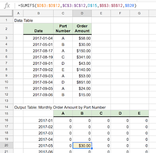
Need help using SUMIFs to match year+month with year+month+date criteria

Hi Google Sheets Wizards!

I am trying to create a monthly summary of how much of a certain part number was sold, so, I'm using SUMIFs to match the part number and the year+month in the Data Table, which shows transactions by part number and by day/date. 

The equation I have for the Output table is: =SUMIFS($D$3:$D$12,$C$3:$C$12,C$15,$B$3:$B$12,$B16). However, this equation only sums the values if the dates are an exact match. The dates in the Output Table are all 2017-XX-01, but formatted to show only the year and month.

My original workaround, which was pretty ugly, was to create a "dummy" column to the right of the Data Table date column and used it to convert the dates to match the first of the month, and then used SUMIFS on that column.

How can I fix my SUMIFs equation to make this work and without having to create that dummy column? What is the cleanest or most elegant solution to what I'm trying to do? I was reading posts about Arrays Formulas, Filter, and Queries, but I've never used those before and they seem much more complicated and might slow my Sheets file down.

Would appreciate any help you guys can provide.

Thank you!!!

Here's the link to the file:

https://docs.google.com/spreadsheets/d/11VupQWS_rwRXS6S3db5FUyUxgSVPP-NLUvywJV4hwdU/edit?usp=sharing

yogi_Compute Duration Between EndTIMEs and StartTIMEs And Compute SUM of Durations Formatted as HH:MM

Google Spreadsheet   Post  #2264

Yogi Anand, D.Eng, P.E.      ANAND Enterprises LLC -- Rochester Hills MI     Oct-10-2017

Question by Margo De Graff

https://productforums.google.com/forum/?utm_medium=email&utm_source=ba_notification#!topic/docs/Kn430jZgQ_s;context-place=mydiscussions

how to format the total duration when hours exceed 24

I want to add up elapsed times, but I don't get Google Sheets to show me the correct answer.

https://docs.google.com/spreadsheets/d/1AO6NHfV2moJBuY7zZlm3KbPxkyMug18OSvP3qHYXCSM/edit?usp=sharing

I tried different types of format, but I can't find a way to get the correct 28:16 result in cell C44.

Am I doing something wrong, or is this a Google Sheet glitch?

yogi_Sort Items In Column A With Hyperlinks On Top

Google Spreadsheet   Post  #2263

Yogi Anand, D.Eng, P.E.      ANAND Enterprises LLC -- Rochester Hills MI     Oct-09-2017

Question by Stefan.B

https://productforums.google.com/forum/?utm_medium=email&utm_source=ba_notification#!topic/docs/6wWmAIpf27k;context-place=mydiscussions

How to sort by cells with hyperlink text in it?

How can I sort the words that have hyperlink (like the example below):

I need your help!

How the list looks	How I would like to sort the list
apple	apple
search engine	search engine
text	numbers
numbers	text
sample text	sample text

My working sheet: https://docs.google.com/spreadsheets/d/10vw5NLAJRGFeWa4yCP_oxgM6hGsRT5lFByMDClIbPms/edit#gid=0

Thaaank youuu for reading my question, I apreciate if you would help me out, please!

yogi_in A2:G2 Show Row By Row Sum Of Entries In Range A3:G

Google Spreadsheet   Post  #2262

Yogi Anand, D.Eng, P.E.      ANAND Enterprises LLC -- Rochester Hills MI     Oct-08-2017

Question by Matheus Castello

https://productforums.google.com/forum/?utm_medium=email&utm_source=ba_notification#!topic/docs/7aLRjRamOJk;context-place=forum/docs
Adding values by row

How can I add up values on the same row without having to do it for every row? Example I want A3 to be = A1 + A2, B3 to be = B1 + B2, C3 to be = C1 + C2 and so forth. Is there any way I can do this without typing it for each row?

Thanks in advance :)

yogi_Rearrange Into Sheet 2 Data From Each Row Of Multiple Columns of Sheet1 Into Rows Of 5 Columns

Google Spreadsheet   Post  #2261

Yogi Anand, D.Eng, P.E.      ANAND Enterprises LLC -- Rochester Hills MI     Oct-07-2017

Question by Luke Terheyden

https://productforums.google.com/forum/?utm_medium=email&utm_source=ba_notification#!topic/docs/Qk2WZVpDLxk;context-place=forum/docs
How to transform one row of a 1000 columns into many rows of 5 columns?

Hi all,

I am trying to turn a strangely formatted table (see below).

At the moment there are more than 1,000 columns with a repeating structure of columns: tool, session, users, length. 

 but I want  to condense this to just 5 columns titled 1.hotel  2. tool 3. sessions 4. users 5. length 

I want the sheet to look like this: 

How do I do this? Thanks!

yogi_Create CALENDAR FOR 12 MONTHS FOR SPECIFIED Year Month And StartDay

Google Spreadsheet   Post  #2260

Yogi Anand, D.Eng, P.E.      ANAND Enterprises LLC -- Rochester Hills MI     Oct-07-2017

post by Rachel Taylor 14, Question by Zuzana Ivanickova

https://productforums.google.com/forum/?utm_medium=email&utm_source=ba_notification#!topic/docs/lt3Z1SXfxaQ;context-place=mydiscussions
Is there a template for the 2018 calendar yet?

This calendar helps a lot. Is there any chance i can have a week starting on monday instead of sunday so we can schedule our weekend tasks entirely?

Thanks in advance.

Zuz